This is the second post on the topic of information entropy. In the first post, we introduced the concept of information entropy, showed how to calculate the entropy for a spectrum, and finally outlined the concept of entropy of the derivative of a signal as a metric to evaluate the ‘jaggedness’ of that signal.
Now, for many practical use cases in visible or NIR spectroscopy, this ‘jaggedness’ is due to noise: random fluctuations of the measured signal that obscure the underlying true signal from the sample. Techniques to smooth noisy spectra are the bread and butter of many preprocessing pipelines. Most smoothing techniques require the adjustment of one or more parameters. The ideal settings of these parameters are those in which random noise is minimised while all information content in a spectrum is preserved. This principle is conceptually simple, but very difficult to use in practice. How do we know which features are noise and which are actual signal?
This is especially tricky for small variations in the spectrum, which may correspond to real responses from the sample, yet be nearly or completely obfuscated by the noise. In the absence of extra information (for instance, repeated measurements), we can’t make up the information that is lost to noise. We can however try to establish a criterion to decide what is the best possible smoothing, given the circumstances.
In this post, I’m proposing a criterion based on a suitable calculation of the information entropy of the derivative of spectra. This figure can be used as a metric to compare different smoothed spectra and establish the optimal set of parameters.
Before we begin, here’s the list of previous posts on spectral smoothing
- Savitzky-Golay smoothing method
- Fourier spectral smoothing method
- Choosing optimal parameters for the Savitzky-Golay smoothing filter
- Wavelet denoising of spectra
- Spectra smoothing with locally-weighted regression
- Optimal spectra smoothing with Fourier ring correlation
And here is, again, the previous post on information entropy, which is required reading for this one.

Information and meaning; signal and noise
Before getting to the main business of this post, we need a brief, but crucial, discussion on terminology.
The term ‘information’ as in ‘information entropy’ or ‘information theory’ is used in the technical sense of ‘amounts of bits’ that are required to encode a signal. As such, there is no difference between ‘signal’ and ‘noise’ in the sense discussed in the introduction. In its technical meaning, information content makes no distinction between ‘useful signal’ and ‘random noise’ insofar as both can be encoded.
Shannon makes this point superbly in the second paragraph of his seminal paper “A Mathematical Theory of Communication” [1] (italic in the original text; emphasis in bold is mine):
The fundamental problem of communication is that of reproducing at one point either exactly or approximately a message selected at another point. Frequently the messages have meaning; that is they refer to or are correlated according to some system with certain physical or conceptual entities. These semantic aspects of communication are irrelevant to the engineering problem.
In purely quantitative terms, information entropy in itself is not useful to distinguish the signal from the noise: they both are information. On the face of it, this is bad news, since distinguishing signal from noise is the main feature of denoising algorithms! However, by using a strategy that is more complicated than simply computing the entropy, we can go some way towards distinguishing signal from noise for the purpose of smoothing a spectrum.
Smoothing with information entropy
Noise generally contains more information (in the technical sense) than signal. The reason was mentioned in the previous post, when we introduced the concept of delentropy (i.e. entropy of the derivative) of a signal. In a normal spectrum there is a natural correlation between nearby points. This correlation is not present in a random signal. Hence, we need fewer bits of information to encode a smooth signal compared to a noisy signal.
It follows that smoothing a spectrum corresponds to decreasing its entropy. However, and at the risk of belabouring this point, we cannot simply look at strategies that minimise the entropy. We would keep smoothing until we get to a flat line, which has minimal entropy! Instead, we need to find an intermediate value of the entropy that corresponds to optimal smoothing.
The approach I propose here requires, in its ideal embodiment, multiple independent repetitions of the same spectrum. These need to be acquired once, for instance on a single sample in a series, and not for every sample.
My idea is to compare the average delentropy of the smoothed signals with the delentropy of the average signal. Assuming that the average signal is the best available approximation to a noise-free spectrum, the optimal smoothing is the one whose delentropy is the closest to the delentropy of the average.
In the specific examples I show below, we use Savitzky-Golay smoothing and we want to find the optimal values of the smoothing window and polynomial order (for more information on these parameters, check the post: Choosing optimal parameters for the Savitzky-Golay smoothing filter).
For each pair of parameters, we will
- Smooth each spectrum in the series.
- Calculate the corresponding delentropy (again, this is the entropy of the first derivative) for each spectrum.
- Calculate the average delentropy of the arrays calculated above.
- Store the delentropy in an array
At the end, we will
- Calculate the delentropy of the average spectrum.
- Compare the last value to each value in the array defined in the previous list.
The pair of parameters that minimises the difference between the two delentropies is the optimal choice.
An example with very noisy spectra
The data for this first example was deliberately acquired for this post. The data set comprises 100 NIR spectra of a black foam collected using the DLP® NIRscan™ Nano evaluation module by Texas Instruments. The data is available for download as a single zipped folder from our GitHub repo.
With start with the imports
|
1 2 3 4 5 6 |
import glob import numpy as np import matplotlib.pyplot as plt import pandas as pd from scipy.stats import entropy from scipy.signal import savgol_filter |
Now load the spectra into an array
|
1 2 3 4 5 |
# Define a list containing file names. Modify the path as required fl = glob.glob("./NIR_black_foam_nirpy/*csv") spectra = np.zeros((len(fl), 228)) for i,j in enumerate(fl): spectra[i,:] = pd.read_csv(j, skiprows=21)['Absorbance (AU)'].values |
ASIDE – If, for any reason, you need the file names in fl to be sorted, you need to use a suitable sorting function. An example is the function proposed by Mark Byers on this StackOverflow post:
|
1 2 3 4 5 6 7 8 |
import re def natural_sort(l): convert = lambda text: int(text) if text.isdigit() else text.lower() alphanum_key = lambda key: [convert(c) for c in re.split('([0-9]+)', key)] return sorted(l, key=alphanum_key) fl = natural_sort(glob.glob("./NIR_black_foam_nirpy/*csv")) |
This is not strictly needed for our purposes, since all the spectra are independent acquisitions from the same sample.
Moving on, here’s the main function implementing the routine described in the first list of the previous section. For each spectrum, this function will loop over a set range of window sizes and polynomial orders (the polynomial order must be strictly positive and strictly smaller than the window size).
|
1 2 3 4 5 6 7 8 9 10 11 12 13 14 15 16 17 18 19 20 |
# Define the array of smoothing window size. window_sizes = np.array([3,5,7,9,11,13,15,17]) # Define entropy array (to be populated) ent_array = np.zeros((spectra.shape[0], window_sizes.shape[0],int(window_sizes.max()) - 1)) for k in np.arange(spectra.shape[0]): # Loop over spectra for i, ws in enumerate(window_sizes): # Loop over window sizes poly_order = np.linspace(1,ws-1,ws-1) # SG filter requires poly_order to be smaller that windows size for po in poly_order: # Loop over poly_order # Smooth spectra. Discard the initial and final points of the spectra. Limit the data in the range 10-200 smoothed_spectrum = savgol_filter(spectra[k,10:200], int(ws),int(po)) # Numerical differentiation of the spectra diff_smsp = np.diff(smoothed_spectrum) # Calculate histogram of the derivatives hist_sm,_ = np.histogram(diff_smsp, bins=smoothed_spectrum.shape[0], density=True) # Calculate delentropy and store it into array ent_array[k, i, int(po) - 1] = entropy(hist_sm, base = 2) # Average over all spectra ent_array_mean = ent_array.mean(axis=0) |
NOTE: The number of bins used in the histogram calculation is somewhat arbitrary. An in-depth discussion on how to choose this value is in this post.
Now we can compare the average delentropy of all spectra with the delentropy of the average spectra.
|
1 2 3 4 5 6 7 8 9 10 11 12 13 |
hist_mean,_ = np.histogram(np.diff(spectra[:,10:200].mean(axis=0)), bins=spectra[:,10:200].mean(axis=0).shape[0], density=True) ent_mean = entropy(hist_mean, base=2) # To find the value of ent_array_mean that is closest to ent_mean, we minimise the absolute value of the difference abs_value_diff = np.abs(ent_array.mean(axis=0) - ent_mean) # Calculate location of the minimum min_loc = np.unravel_index(np.argmin(abs_value_diff), abs_value_diff.shape) # Print minimum and its location print(np.min(abs_value_diff), min_loc) # Define an array that contains all possible values of poly_order poly_o = np.linspace(1, window_sizes.max() - 1, window_sizes.max() - 1) |
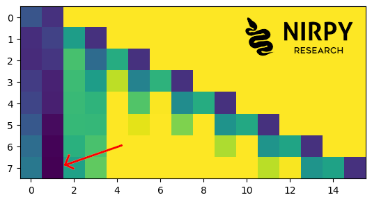
The array abs_value_diff is the absolute difference between the average delentropy of all spectra with the delentropy of the average spectra. The minimum of this array will correspond to the conditions in which the two delentropies are closest. The code above will print the value of the minimum and its location. In my case, the location is (7,1) , which are the indices of window_sizes (17) and poly_o (2) respectively, that minimise the difference.
You can also plot the heat map of abs_value_diff array with a suitable max value, to make sure you can distinguish small difference between the pixels. In the map below, all the pixels above the max value are displayed as yellow, so that we can distinguish small difference between the other pixels.
Finally, we can plot a comparison between original and smoothed spectra, by choosing the spectrum number 80 as an example.
|
1 2 3 4 5 6 7 8 9 10 11 12 13 14 15 16 17 18 |
ws = window_sizes[min_loc[0]] po = int(poly_o[min_loc[1]]) sn = 80 with plt.style.context(('seaborn-v0_8-whitegrid')): fig, ax = plt.subplots(2,1, figsize=(6, 9)) ax[0].plot(spectra[sn,10:200], lw=2, label = 'Spectrum 80, original') ax[0].plot(savgol_filter(spectra[sn,10:200], ws,po), lw=2, label = 'Spectrum 80, smoothed') ax[1].plot(spectra[:,10:200].mean(axis=0), lw=2, label = 'Avg of original spectra') ax[1].plot(savgol_filter(spectra[:,10:200], ws,po, axis=1).mean(axis=0), lw=2, label = 'Avg of smoothed spectra') ax[0].set_ylabel("NIR absorbance", fontsize=14) ax[0].set_xlabel("Wavelength index (arbitrary units)", fontsize=14) ax[1].set_ylabel("NIR absorbance", fontsize=14) ax[1].set_xlabel("Wavelength index (arbitrary units)", fontsize=14) ax[0].legend() ax[1].legend() ax[0].set_title("Optimal smoothing", fontsize=16) plt.show() |

Looking at the top chart alone, it’s difficult to judge whether the smoothed spectrum is ‘smooth enough’. By using the delentropy approach, we end up with a result that reproduces very well the important features, as proven by the bottom chart that shows the averages. The broad variations (on a larger scale) are preserved, while the jaggedness (due to noise) is removed.
As a final note, the maximum value for the window size was chosen to be 17. We could potentially increase that value, but at higher values the savgol_filter function runs into problems during the fit procedure.
A more realistic case
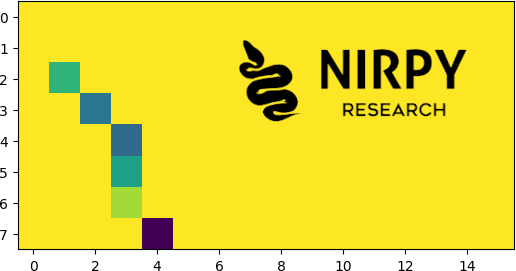
I’ve applied the code above to the more realistic case of NIR spectra from fresh avocadoes. The spectra were acquired using the same instrument and are also available as a zip folder on our Github repository. This case is more realistic since the samples produce a much stronger NIR signal. In this case the optimal smoothing is achieved with window size of 17 and polynomial order of 5. Here’s the heat map obtained with exactly the same code:
And here’s the spectra comparison, using the spectrum number 10 as an example:
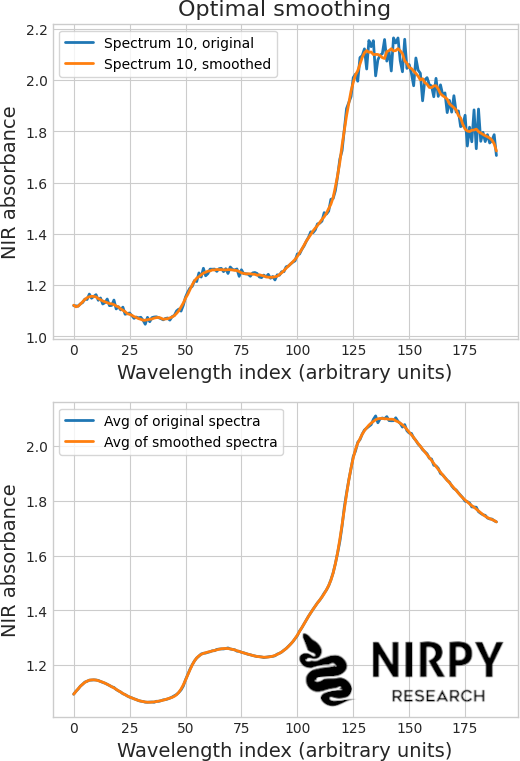
It’s interesting to note how, the smoothed spectra are still quite noisy, especially towards the end. Intuitively, I would have, perhaps, smoothed the spectra more. However, the delentropy method produces results that, once averaged, are extremely close to the average spectrum, without distortions.
Stronger smoothing would be sub-optimal, since it would distort some of the relevant features in the spectrum, as in the plot below.

Conclusions
This is the second installment of our mini-series on defining a smoothing criterion based on the information entropy. An additional technical note on the histogram calculation is available here. Admittedly, I feel I just scratched the surface on this topic, and there is so much more I’m going to think about. As always, I’m keen to hear comments or feedback. For now, thanks for reading and take care!
References
[1] C. E. Shannon (1948). “A Mathematical Theory of Communication”. Bell System Technical Journal, 27, 379-423. [PDF]
**
Feature image by Agostino Aglio (1831–48), “Facsimile of the Codex Bodley, ca. before 1521“, featured on Public Domain Review in the collection Antiquities of Mexico (1831–48). Image sourced from the Public Domain Image Archive / Internet Archive / Smithsonian Libraries and Archives.