Last update:
This is an introductory post on the concept of information entropy, or Shannon information. I plan to build on this concept to define, in the next post, another approach to optimise the parameters of smoothing filters, such as the Savitzky-Golay. That’s right, despite discussing spectra smoothing many times on this blog, I’m still thinking about principled approaches to establish the optimal way of smoothing.
But let’s go step by step. In this first post we will:
- Introduce the concept of information entropy (sometimes, we refer to it simply as entropy, keeping in mind that it is separate from the thermodynamics concept of entropy, not discussed here).
- Calculate the entropy for a NIR spectrum.
- Discuss an important extension of the concept of information entropy, which will be key for future discussions on spectra smoothing.

Information entropy
The concept of information entropy was first introduced by Claude Shannon in his seminal 1948 paper “A Mathematical Theory of Communication” [1]. Now, as the title of the paper suggests, Shannon was interested in communication of signals through noisy channels. A signal must go from a sender to a receiver, and it may be corrupted by random noise during transmission. How can we quantify the amount of information in this signal? In other words, what is the minimum amount of bits (on/off switches) that are needed to encode the signal? Also, how much information is lost in the process of noisy transmission, and how to make sure that redundancies are built in the communication protocol to correct for the lost bits?
To answer these types of questions, Shannon ended up developing the concept of information content in a signal (information entropy, or Shannon entropy). We won’t cover all the topics mentioned in the previous paragraph, but we’ll review the key concepts of information entropy, preparing the ground for the next, more specific, post on spectra smoothing.
Using the language of statistical analysis, let’s consider a random variable A which can generate a number of outcomes. We call a one such outcome and we assign the probability p(a) to the realisation of outcome a (in assigning the probability p(a) to a, we are implicitly assuming that the probability distribution of the random variable A is known. We’ll return to this key assumption very soon). For instance, the random variable is a conventional die, whose outcomes are the values from 1 to 6, each with equal probability p = 1/6.
With these preliminaries out of the way, we can define the information content of the outcome a as
h(a) = \log_{2} \frac{1}{p(a)} = -\log_{2} p(a).The information content is proportional to the inverse of the probability. In other words, h(a) is the level of surprise we may experience at observing the outcome a. Rare events, i.e. events that have low probability, have larger information content. Conversely, high-probability outcome are (by definition!) to be expected and bring little or no surprise.
The information entropy is the weighted sum of the information contents of each outcome:
H(A) = \sum_{a} p(a) h(a) \log_{2} = - \sum_{a} p(a) \log_{2} p(a),where the sum is to be performed on each outcome a of A. As anticipated earlier, the probability p(a) must be known in advance for these definitions to strictly apply.
However, if p(a) is not known, it could be estimated from the signal itself, as the (suitably normalised) number of occurrences of each value in a signal.
Calculating the information entropy
The key function for the entropy calculation is scipy.stats.entropy available from SciPy.
Here’s an example of its usage. For the purpose of this example, we load some spectra from our GitHub repo and calculate the entropy for one of them.
|
1 2 3 4 5 6 7 8 9 10 11 12 13 14 15 16 17 |
import numpy as np import pandas as pd from scipy.stats import entropy # Load data url = 'https://raw.githubusercontent.com/nevernervous78/nirpyresearch/master/data/peach_spectra_brix.csv' data = pd.read_csv(url) # Extract spectra arrays X = data.values[:,1:].astype("float32") # Calculate normalised histogram of the first spectrum hist_s1,_ = np.histogram(X[0,:], bins=X.shape[1], density=True) # Calculate entropy of the spectrum ent = entropy(hist_s1, base = 2) print(ent) |
The key step is to calculate the histogram of the spectrum. This is the array we need to pass to the scipy.stats.entropy function, not the spectrum itself. The way I’ve done it here is by using the numpy.histogram function and setting density=True to have the result normalised. In this way, the sum of the elements of the histogram array is 1, making it a suitable (empirical) probability distribution for the entropy calculation.
Note that the result would be slightly different is we were to choose a different number of bins. I set it to be equal to the dimensionality of the spectrum, which is 600 in this case. I could choose any number of bins up to 600 and the resulting entropy will generally decrease as we decrease the number of bins. This reflects the fact that by reducing the number of bins, more and more similar values will be binned together, thus reducing the information content of the individual wavelength bins. The choice of the number of bins is somewhat arbitrary, but this is not an issue for our purpose, which will be that of comparing results between different smoothing parameters, as long as the number of bins is the same for all cases.
A potential issue
So far so good, but there is a potential problem. Since the entropy calculation relies on the histogram, the actual order in which the values appear in the spectrum array is immaterial. For instance, consider the plot of the spectrum we used in the calculation above, and a version of it in which the values are randomly shuffled.
|
1 2 3 4 5 6 7 8 9 10 11 |
rng = np.random.default_rng() with plt.style.context(('seaborn-v0_8-whitegrid')): fig, ax = plt.subplots(2,1, figsize=(5, 10)) ax[0].plot(X[0,:], lw=2) ax[1].plot(X[0,rng.permutation(X.shape[1])], lw=2) ax[0].set_xlabel("Wavelength index", fontsize=14) ax[0].set_ylabel("NIR Reflectance", fontsize=14) ax[1].set_xlabel("(Randomized) Wavelength index", fontsize=14) ax[1].set_ylabel("NIR Reflectance", fontsize=14) plt.show() |
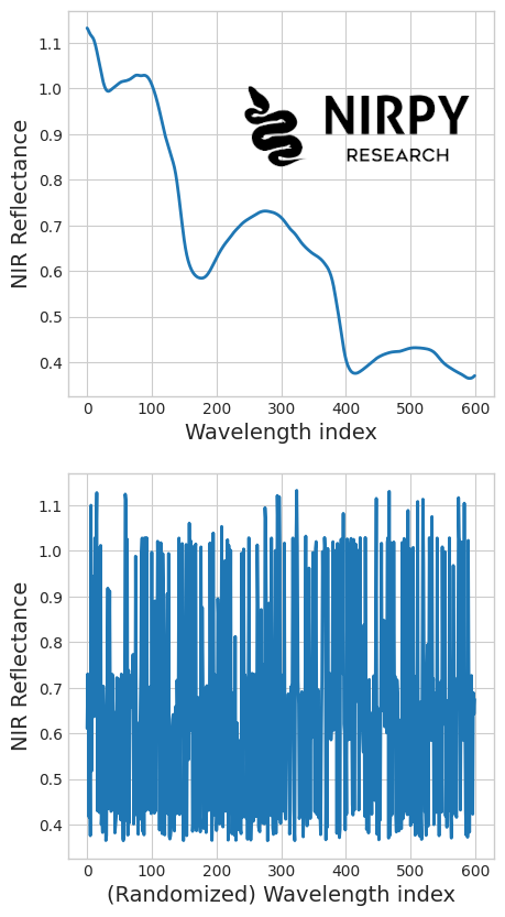
These two ‘spectra’ have the same entropy (as we will verify later in this post), since they have the same histogram. However, you’d be very surprised if your spectrometer would output the spectrum at the bottom of the previous figure, rather than the spectrum at the top. We used the word ‘surprise’ to describe the information content of an outcome: unexpected outcomes have higher information content.
There is a sense then, in which we would expect a measure of surprise associated with the randomised spectrum to be higher than the same measure for a ‘normal’ spectrum. The information entropy, as defined above, cannot be used as one such metric. But fear not! There is a small adjustment that enables us to define such a order-dependent metric.
Entropy of the derivative of a spectrum
The small adjustment we need to do is to compute the information entropy of the first derivative of the spectrum, rather than of the spectrum itself. I learned this concept from a paper by Kieran Larkin [2] (and from discussions with Kieran himself). The starting point for Kieran’s work was to extend the concept of Shannon entropy to two dimensions, i.e. for image processing.
In doing so, Kieran defined a ‘second order entropy’ which he dubbed delentropy, it being the entropy of a signal’s gradient. This approach can be naturally extended to 2D by calculating the entropy of the gradient of an image. In our case, we don’t need to go that far, and just stick with the notion of entropy of the derivative of a 1D signal.
Calculating the entropy of the first derivative accounts naturally for the shape of the spectrum. Take another look at the figure above. In the normal spectrum (top chart) there is a natural correlation between nearby points; roughly speaking, the spectrum is continuous. This correlation is not present in the bottom graph, where the operation of randomising the order has destroyed the natural correlation and the resulting signal is jagged.
The first derivative of the ‘normal’ spectrum will contain values that are not too large (in magnitude) since the spectrum is rather smooth. Conversely, the derivative of the randomised spectrum will contain much larger values (again, in magnitude) and much larger variations between the values.
Therefore, the entropy of the first derivative will be naturally lower for the normal spectrum than the same metric calculated for the randomised spectrum.
Before doing the actual calculation, and as an aside, I just wanted to add that the ‘natural correlation’ between nearby points in a spectrum, is what we often called ‘collinearity‘. This is a problem in regression (hence the need for some sort of decomposition), but it’s the reason why a spectrum can be reconstructed sufficiently well by a relatively small number of principal components.
OK, time to write the code.
|
1 2 3 4 5 6 7 8 9 10 11 12 13 14 15 16 17 18 19 20 21 22 23 24 25 |
rng = np.random.default_rng() # Calculate histogram of the normal spectrum hist_s1,_ = np.histogram(X[0,:], bins=X.shape[1], density=True) # Calculate histogram of the randomised spectrum hist_s2,_ = np.histogram(X[0,rng.permutation(X.shape[1])], bins=X.shape[1], density=True) # Calculate corresponding entropies ent_1 = entropy(hist_s1, base = 2) ent_2 = entropy(hist_s2, base = 2) print(ent1, ent2) # First derivative of the normal spectrum Xd = np.diff(X[0,:]) # First derivative of the randomised spectrum Xrd = np.diff(X[0,rng.permutation(X.shape[1])]) # Histograms hist_d1,_ = np.histogram(Xd, bins=Xd.shape[0], density=True) hist_d2,_ = np.histogram(Xrd, bins=Xrd.shape[0], density=True) # Entropies ent_d1 = entropy(hist_d1, base = 2) ent_d2 = entropy(hist_d2, base = 2) print(ent_d1, ent_d2) |
The code above prints the result of the entropy calculations for the spectra, and for the derivatives. In the first case the two results are identical (since the histograms are identical). In the second case, the entropy of the gradient of the randomised spectrum is larger than the corresponding entropy of the gradient of the normal spectrum. This reflects the loss of correlation of the randomised spectrum, compared to the normal one.
Looking ahead
In the next post, we will see how we can use the entropy of the first derivative of a spectrum to establish a natural criterion for smoothing it. This will be applicable every time we have a group of similar spectra, for instance many repetitions of the same measurement, or measurements of different samples under identical conditions. This is not too restrictive, since it corresponds to most practical uses of NIR or optical spectroscopy aided by chemometrics.
Thanks for reading, and until next time.
Daniel
References and credits
[1] C. E. Shannon (1948). “A Mathematical Theory of Communication”. Bell System Technical Journal, 27, 379-423. [PDF]
[2] K. G. Larkin (2016). “Reflections on Shannon Information: In search of a natural information-entropy for images”. arXiv:1609.01117v1 [PDF]
**
Feature image by Agostino Aglio (1831–48), “Facsimile of the Codex Bodley, ca. before 1521“, featured on Public Domain Review in the collection Antiquities of Mexico (1831–48). Image sourced from the Public Domain Image Archive / Internet Archive / Smithsonian Libraries and Archives.