Optimal spectra smoothing with Fourier ring correlation

In a pair of previous posts, I discussed one of the most common smoothing methods for spectra, namely the Savitzky–Golay technique. The first post introduced the topic, while the second post discussed how to choose the optimal parameters for the Savitzky–Golay (SG) filter. Other posts on spectra smoothing are:

• Fourier spectral smoothing
• Wavelet denoising
• Locally-weighted regression

Common to all of these methods is the issue of how to choose the smoothing “strength”. This was specifically discussed in my second post on the SG filter. In this post I come back to this topic with a different approach, adapting the concept of Fourier ring correlation used in imaging. I believe one could use this idea to estimate the best way to smooth a spectrum given its noise level.

The problem of optimal smoothing

Smoothing a spectrum aims at removing as much as possible of the noise component, while at the same time preserving as much as possible of the information. By “information” I mean the spectral variations that are related to the sample and not to randomness of the measurement process.

This is easier said than done of course. In my second post on the SG topic, I proposed that a way to achieve this goal would be to look at a portion of the spectrum which is, for the most part, devoid of important features. That might enable a reasonable estimate of the noise level in the spectrum by means of the ‘power spectrum’, which is the squared magnitude of the Fourier transform of the original spectrum. Subtle changes in the SG filter parameters can be visualised in the power spectrum, as a way to more objectively set the optimal smoothing for the spectra.

In essence, the idea is to have a way to automatically and quantitatively estimate the noise, in a way that is independent on the specific experiment. This is in the spirit of avoiding the following:

1. Subjectively judging what the “right” amount of smoothing is by eye. No matter how good I am (or I think I am) at making these decisions, I’d like a programmatic way to smooth data, (eventually) without human intervention.
2. Optimising the smoothing parameters as a part of the model prediction pipeline. Much as it is tempting to choose the parameters which gives us (say) the best RMSE on a regression problem, this might represent a risk of overfitting, especially (and that is often the case) when the data comes from a single spectrometer or a single experiment.

This post is a further step further in this work. The “power spectrum” approach still requires a subjective judgement (or previous knowledge) of what is a region “devoid of features” and how well the spectrum of the noise is suppressed. By adding some more data to the mix, we can however do the same thing in a more principled way, and that works for every spectrum regardless of the sample measured or the instrumentation used.

The idea is borrowed from the field of microscopy, which very often requires to estimate the resolution of an imaging system. Resolution is a bit of a fuzzy concept, especially at very high resolutions where noise plays a very important role. One of the widely used methods for spatial resolution estimation is called Fourier Ring Correlation (FRC) which can be easily applied to spectroscopy as well. Here’s how.

Fourier Ring Correlation

As the name suggests, FRC has to do with Fourier transforms and, hence, power spectra. Here we assume that you are familiar with these concepts. You are welcome to go back and read my previous post on power spectra or, in fact, just about any good book/post on Fourier transforms.

The idea of FRC (sometimes called Fourier shell correlation for 3D imaging) goes like this. Suppose you take two images in exactly the same conditions (for instance with a microscope). The two images will be identical except for the random noise that is inevitably present. The random noise has high spatial frequency (i.e. it changes rapidly from one pixel to the next). This can be visualised in the power spectra of the two images: the power spectra will be identical at low Fourier coordinates (low spatial frequencies) and become different at high spatial frequencies.

Hence, if we calculate a correlation between the Fourier transform of the images, as a function of the Fourier coordinate, we expect to observe high correlation that drops to zero as we increase the spatial frequency. This type of correlation is precisely what we called Fourier ring correlation. The reference to a “ring” has to do that for a 2D Fourier transform, the locations of points that have the same spatial frequency is a ring. The actual formula looks like this

FRC(q) = \frac{\sum_{q \in \mathrm{ring}} F_1(q) \cdot F_2(q)^{\ast} }{(\sum_{q \in \mathrm{ring}} \left|F_1(q)\right|^2) (\sum_{q \in \mathrm{ring}}\left|F_2(q)\right|^2)}

where F_1(q) and F_2(q) are the Fourier transforms of image 1 and image 2 respectively, and the asterisk means complex conjugation. The denominator of the above expression serves as a normalisation factor so that the correlation will be bound between 0 and 1.

To apply this concept to spectral smoothing, we would like to adapt the formula from 2D (or 3D) to one dimension only. The formula is easy enough to write, as we don’t need to sum over all elements on a ring, but just consider the product of the (unique) elements at Fourier frequency q

FRC(q) = \frac{F_1(q) \cdot F_2(q)^{\ast} }{( \left|F_1(q)\right|^2) (\left|F_2(q)\right|^2)}.

In addition, since the Fourier transform of an array of size N will only have N/2 independent elements, we only need to calculate the above formula for N/2 elements.

A Python function (using numpy) for the above formula looks like this

The inputs are the two Fourier transforms  Xf1  and  Xf2  of size N and the output is an array of size N/2. Importantly, keep in mind that Fourier transform arrays are usually complex, hence we need to take the real part of the outputs before returning their values. There is another important difference between our case and the 2D case, and we’ll explain it as we work through the example below.

Fourier ring correlation of one-dimensional spectra

To work through the procedure, we use a dataset of 500 NIR spectra of ABS plastic available at our Github repo. I have deliberately set the acquisition parameters to get noisy data, which will give us the opportunity to study the effect of smoothing filters on the FRC. Let’s start with the imports

Let’s load the data and calculate the 1D fast Fourier transform (FFT), spectrum by spectrum

Now we plot one spectrum and the corresponding power spectrum

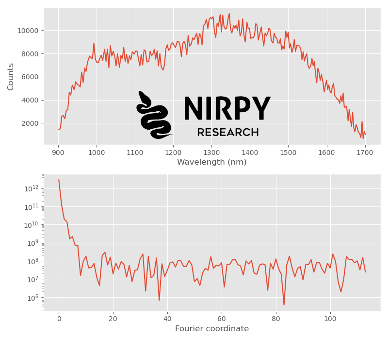
As anticipated, the spectrum is very noisy. The corresponding power spectrum drop to the noise level pretty quickly, at about the tenth element of the arrays. This becomes even clearer if we plot two power spectra, corresponding to the the first and the 100th NIR spectra

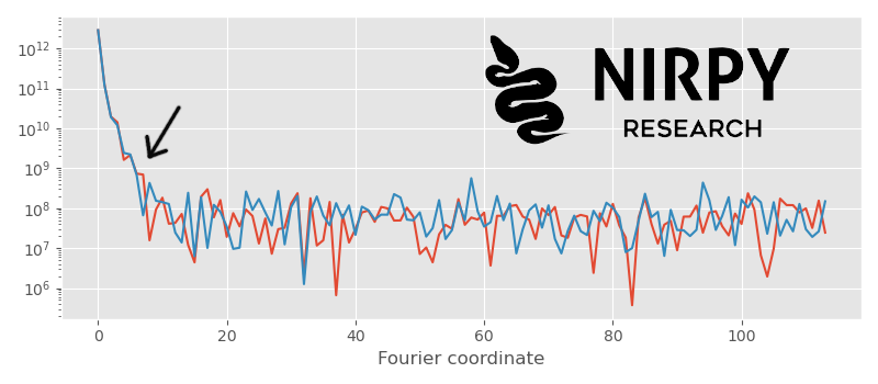
The two power spectra are well correlated up to about the position of the arrow. This corresponds to the overall shape of the spectra. The details however are noisy, so the two power spectra are essentially random for larger Fourier frequencies.

What we have just described in word is the idea that FRC quantifies: the correlation of two Fourier transforms as a function of the Fourier coordinate.

In principle, we could just go ahead and apply the function above to the two Fourier transforms Xf[0,:] and Xf[100,:] . The problem however is that just two spectra can exhibit spurious correlations just because of randomness. This usually doesn’t happen for 2D images because there are many Fourier coordinates in any ring, and these are summed together. This generally gets rid of any spurious correlation. In 1D we only have two components to multiply and spurious correlation do appear and are significant.

This is the main difference between the 2D case and the 1D case, that we anticipated at the end of the previous section. To remedy this issue we average the FRC calculation over a large number of spectra. We pick a number of spectra (say, 50), we calculate the FRC over  all possible pairs,a nd we average the result.

The code may look like this

Here it is: the correlation is near perfect for the first 2-3 elements and drops rapidly to zero after about the tenth-twelfth Fourier coordinate.

Optimal denoising strategy guided by Fourier ring correlation

OK, so how do we use this information to guide our denoising strategy?

A way to interpret the FRC plot above is to say that the useful information in every power spectra is only up to about the tenth or twelfth element. Let’s call this value a cut-off, after which the power spectra are it’s noise. Therefore, the optimal denoising filter will remove everything above the cut-off, but leave unchanged everything below that value.

Let’s check this with a Gaussian smoothing. Let’s apply a Gaussian filter with \sigma = 1 to our spectra and see what happens to the FRC

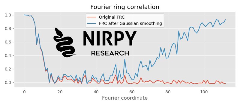
What’s going on here? The FRC of the smoothed spectra is identical to the original FRC at low Fourier coordinates. It drops to zero, but then starts to rise again! This increase is an artefact of the smoothing: as the Gaussian filter suppresses higher spatial frequencies, the spectra (which were initially uncorrelated at high frequencies) start to be correlated by virtue of the convolution with an identical filter.

This “artefact correlation” kicks in at about the 50th Fourier coordinate. In other words, a Gaussian filter with \sigma = 1 removes noise from about the 50th Fourier coordinate onwards.

Given that our spectra are very noisy, we could make the Fourier filter stronger (smooth more) without losing information. The idea is that the \sigma of the Gaussian needs to be tuned until the artefact correlation approaches the cut-off. If we repeat the code above with \sigma = 2 we get

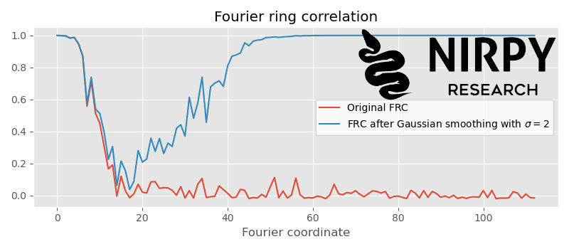
That’s about the right amount of smoothing. The artefact correlation appears at around the cut-off position. If we would smooth more, say \sigma = 3 , the artefact correlation would start to overlap with the actual correlation

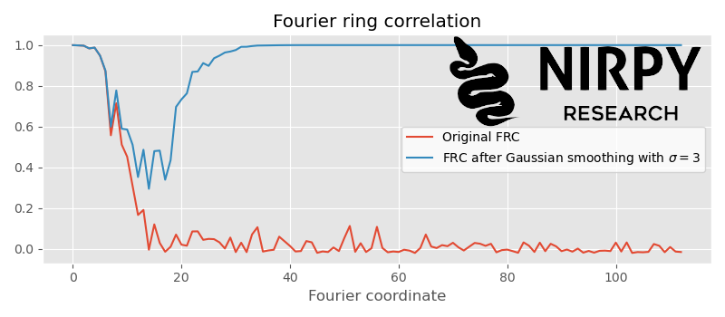
This means our smoothing filter is now altering useful information in our spectra and we need to reduce its strength.

Fourier ring correlation with Sav-Gol filter

In the example above, I used a Gaussian filter as it produces a monotonic suppression of the signal in Fourier space. This corresponds to a monotonic increase of the “artefact correlation” in the FRC.

An SG filter is different, as it is designed to smooth a spectrum based on a polynomial fit on each contiguous region in spectrum itself. The size of the region is defined as the “window” and the larger the window, the stronger the smoothing will be. However, the fact that we define a window, will generate a non-monotonic signal in Fourier space.

Suppose we start with a window of 5 and run this code (same as above except for the SG filter)

Now the artefact correlation is a peak, corresponding to the first position in Fourier space where the window of the SG filter is completely suppressing the signal.

Given that the artefact correlation is far enough from the actual correlation, we can increase the window further. If we set w to 11 we get

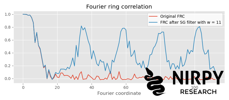
Now the artefact correlation is periodic (for the more mathematically-inclined, this has to do with the fact that the Fourier transform of a top-hat function is a sinc function which drops to zero periodically in Fourier space) but for our purposes is enough to check that it kicks in after the cut-off. This would be about the right amount of smoothing to apply to our spectra.

Note how this is defined by the amount of noise in the spectra. Suppose we were to start with a lower level of noise (which we can simulate by averaging every 10 spectra in our list of 500 spectra)

The same SG filter with a window of 11 would now be too harsh
The actual Fourier ring correlation (red curve) now extends up to about the 40th Fourier coordinate (meaning the level of noise in our spectra is reduced), and the SG filter is suppressing useful information! In these (improved) noise conditions we should reduce the amount of filtering to make the most of the predictive ability of our machine learning algorithms!

As always, thanks for reading until the end and until next time.

Daniel