This is the third post on the topic of information entropy. In the first post, we introduced the concept of information entropy, showed how to calculate the entropy for a spectrum, and finally outlined the concept of entropy of the derivative of a signal as a metric to evaluate the ‘jaggedness’ of that signal. In the second post, we applied this method to establish a criterion for optimal smoothing.
In this post, we add a technical note on the calculation of entropy, and more specifically on the calculation of the histogram of a signal. Following a suggestion from a reader of the blog, I realised that the arbitrary choice of selecting the number of bins has an effect on the result.
In this post, we discuss this technical point in some depth.

The issue
Let’s recap the main steps to calculate the information entropy (see the first post on the topic for the details).
- Use the scipy.stats.entropy function available from SciPy.
- Calculate the histogram of the spectrum.
- Apply the entropy function to the histogram.
Here’s the code snippet we included in the first post, as an example. The spectra are taken from our GitHub repo, and we calculate the entropy for one of the spectra.
|
1 2 3 4 5 6 7 8 9 10 11 12 13 14 15 16 17 |
import numpy as np import pandas as pd from scipy.stats import entropy # Load data url = 'https://raw.githubusercontent.com/nevernervous78/nirpyresearch/master/data/peach_spectra_brix.csv' data = pd.read_csv(url) # Extract spectra arrays X = data.values[:,1:].astype("float32") # Calculate normalised histogram of the first spectrum hist_s1,_ = np.histogram(X[0,:], bins=X.shape[1], density=True) # Calculate entropy of the spectrum ent = entropy(hist_s1, base = 2) print(ent) |
The key issue is the choice of the number of bins, which in the code above is set to be equal to the length of the spectrum. However, as pointed out to me by Philip Wilson, this choice is arbitrary, and in fact, it affects the final calculation. Is there a way to improve this step?
A possible way out
The information entropy is defined as the weighted sum of the information contents of each outcome a of a random variable A:
H(A) = \sum_{a} p(a) h(a) = - \sum_{a} p(a) \log_{2} p(a),where the sum is to be performed on each outcome a of A. The formula depends on the probability p(a) of each outcome, and it implies that the probability must be known in advance.
Of course, in all practical cases, p(a) is unknown. Therefore, we must estimate it from the data, but calculating the histogram of the signal, suitably normalised. The histogram is calculated by defining a number of bins, that is a number of intervals from the minimum to the maximum of that signal.
Let’s calculate the entropy as a function of the number of bins, for a series of spectra.
|
1 2 3 4 5 6 7 8 9 10 11 12 13 14 15 |
# Load data url = 'https://raw.githubusercontent.com/nevernervous78/nirpyresearch/master/data/peach_spectra_brix.csv' data = pd.read_csv(url) # Extract spectra arrays X = data.values[:,1:].astype("float32") ent_array = np.zeros((spectra.shape[0], 50)) nbins = np.logspace(1,6,50) for k in np.arange(X.shape[0]): for j, nb in enumerate(nbins): # Calculate entropy with a variable number of bins hist_sm,_ = np.histogram(X[k,:], bins=int(nb), density=True) ent_array[k, j] = entropy(hist_sm, base = 2) |
We store the calculated entropy results in a 2D array ent_array as a function of the number of spectra and the number of bins. For reference, the array X has dimensions 50×600, that is 50 spectra, each with 600 wavelength points. Now, let’s calculate the average and standard deviation of the entropy array along the first axis (the number of spectra).
|
1 2 |
ent_array_mean = ent_array.mean(axis=0) ent_array_std = ent_array.std(axis=0) |
This produces the average and the standard deviation of the entropy array as a function of the number of bins used for the histogram calculation. We can now plot the results
|
1 2 3 4 5 6 7 8 9 10 |
fig, ax1 = plt.subplots(figsize=(7, 4)) line1, = ax1.loglog(nbins, ent_array_mean, color='k', linewidth=2, label="Mean Entropy") ax1.set_ylabel("Mean Entropy", fontsize=12) ax1.set_xlabel("Number of Bins", fontsize=12) ax2 = ax1.twinx() ax2.set_ylabel("Entropy Standard Dev.", fontsize=12) line2, = ax2.loglog(nbins, ent_array_std, color='r', linewidth=2, label="Entropy Std") plt.show() |
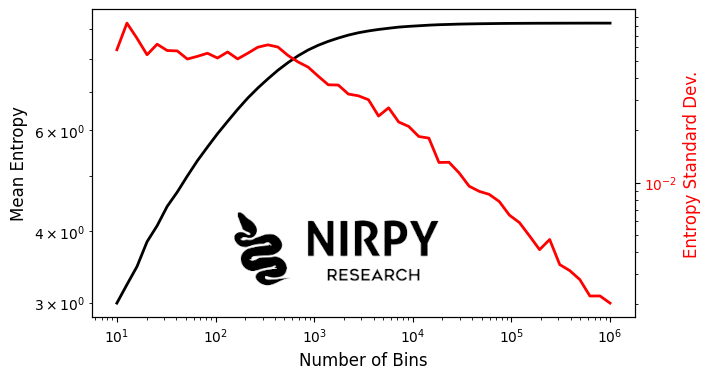
Calculating the histogram with a large number of bins corresponds to finely sampling the spectrum. I initially thought this to be a good idea, since the mean entropy is converging! As Philip Wilson (thanks, Philip!) correctly pointed out however, this is deceptive, since it corresponds to sampling each value exactly once. The limit value is just log_{2}600 \approx 9.23 . In other words, the entropy is the same for all spectra, since we ended up making p(a) = 1/600 for all spectra.
If we look at the standard deviation, however, we see that its value is roughly constant up until 200 bins, and it decreases afterwards. Note that we are making this calculation on a sample of 50 independent spectra, for which we expect the value of the entropy to be sample-dependent. The value of the standard deviation reflects this fact, but after 200 bins, the individual elements of the entropy array become more and more similar to each other (standard deviation becomes smaller and smaller). Therefore, the largest value at which we are meaningfully sampling the histogram is approximately 200. This would be, in this case, the optimal number of bins for the entropy calculation.
Conclusions
The conclusion of this exercise, is that the code in the previous two entropy posts must be slightly modified. The number of bins used in the histogram calculation must be set to the value after which the standard deviation of the entropy array starts decreasing.
**
Feature image by Agostino Aglio (1831–48), “Facsimile of the Codex Vindobonensis, ca. late 15th or early 16th century“, featured on Public Domain Review in the collection Antiquities of Mexico (1831–48). Image sourced from the Public Domain Image Archive / Internet Archive / Smithsonian Libraries and Archives.