
Last update:
We’re back to one of our favourite topics at Nirpy Research. We discussed spectra smoothing in many flavours in the past, and discussing the locally-weighted regression approach will help, I hope, in improving the understanding of them all. A few examples form past posts are:
- Savitzky-Golay smoothing method
- Fourier spectral smoothing method
- Choosing optimal parameters for the Savitzky-Golay smoothing filter
- Wavelet denoising of spectra
Amongst these, the Savitky-Golay filter has been the most popular one, on this site and (arguably) in many applications. For this reason, I may as well give away the punch line: the Savitky-Golay (SG) filter is an example of locally-weighted regression.This post will explore the concept further, in the process, explain and generalise the concept of curve smoothing with locally-weighted regression, and it’s divided into two main parts:
- The basics of locally-weighted regression
- An example of spectra smoothing with locally-weighted regression in Python.

Locally-weighted regression: the basics
Historically, locally-weighted regression techniques have been developed for “scatterplot smoothing”. Think of a scatter plot: a cloud of data points, more or less noisy, distributed in a 2D chart. If we wanted to fit a curve to these points we have two choices:
- Parametric regression. This is the conventional regression approach we know and love. Assume a functional dependence (for instance linear, or quadratic) and estimate the parameters of this function with (say) a least-square minimisation. The regression is called parametric because a functional form is chosen (and thereby fixed), and we only estimate its parameters free parameter. So, for instance, we could assume a linear dependency y = a x + b and estimate its parameters a and b using least-squares minimisation.
- An alternative approach is to use a non-parametric regression, such as the SG filter. This approach doesn’t assume a functional dependency at all and therefore doesn’t aim at estimating global parameters. For every point in the scatter plot (or in a spectrum), it performs a polynomial regression in the neighbourhood of that point and replace the given point with the result of this local regression calculated at the same position. Note that, despite its name, we still have a few parameters to tweak, but these refer to the local(ly-weighted) regression rather than the global one. So for instance, the SG filter will require specifying the order of the polynomial, or the size of the neighbourhood over which to perform the local regression.
The main advantage of a parametric regression is that once its parameters have been estimated, we don’t need to look at the data again. Once we fit a (say) PLS model to a bunch of spectra, we just need to save the parameters of that model, not the spectra. The parameters are enough to predict the results of the regression on a new (previously unseen) spectrum. The main limitation of the approach, on the other hand, is that a functional dependency must be assumed, and this not always possible for complicated wave forms.
Conversely, locally-weighted regression can fit any wave form regardless of its specific shape, but every time a new fit is done, we need to know the underlying data. That is to say, for instance, that the result of an SG filter on a spectrum are calculated every time from scratch, and we need the original data every time.
That’s about it, but before moving on, let’s briefly discuss some terminology and give some references. Given its inception is “scatterplot smoothing”, locally-weighted regression is also referred to as LOESS (locally estimated scatterplot smoothing) or LOWESS (locally weighted scatterplot smoothing). More info on this can be found on the Local Regression Wikipedia page. See also Refs. [1-2] for some relevant papers.
One final thing. The “weights” in the locally-weighted regression refer to a weight function that is used to define the extent of the neighbourhood of one point. Traditionally, the tri-cubic function w(d) = (1 - |d|^3)^3 is used, whereby d, defined in the interval [0,1], is the distance from the point of interest (i.e. around which we want to compute the local regression).

Spectra smoothing by locally-weighted regression in Python
Our implementation of locally-weighted regression is based on the LOWESS smoother provided in the statsmodel package. All we need is these imports
import numpy as np
import pandas as pd
import statsmodels.api as sm
Next, let’s load the data and select one spectrum. Note: this dataset is will be available soon at our Github page.
data = pd.read_csv("../data/nir_cucumber.csv")
X = data.values[:,4:].astype("float32")
wl = np.array(data.keys()[4:].astype('float32'))

lowess = sm.nonparametric.lowess
z = lowess(X[0,:], wl, frac=0.02, it=2, return_sorted=False)

plt.plot(wl, X[0,:], 'k', label = 'data')
plt.plot(wl, z, 'r', label = 'lwr')
plt.xlabel("Wavelength (nm)")
plt.ylabel("NIR Reflectance")
plt.legend()
plt.show()
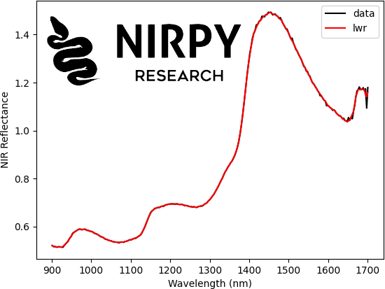
As you can see, the lowess function requires a spectrum (the y-variable), the wavelength range (the x-variable), a frac parameter, defined between 0 and 1, which determine the width of the weight function, and an it parameter which determines how many smoothing iterations are performed. Increasing either frac or it will result in a smoother curve.
Here you can note an important difference between the SG filter and the LOWESS filter. The latter requires the wavelength (or wavenumber, etc) information. This is an important point, as in many cases the spectra;l points are not equally spaced in the wavelength range, so that spacing between the points tend to increase with increasing wavelength. This is not accounted for in the SG filter, which requires only the spectra, but it is naturally taken into account in the LOWESS implementation.
On the other hand, the Scipy implementation of the SG filter which we use all the time here, can perform derivatives and smoothing in one go, which is handy when dealing with many types of smooth spectra such as NIR spectra. Since we are here, let’s write a utility function to perform derivative smoothing with the LOWESS approach.
Derivative smoothing with locally-weighted regression
Our task is to implement a function performing a numerical differentiation (to the first or the second order) followed by a LOWESS smoothing. Naively, we could use the numpy.diff function to perform the differentiation, but, as explained at length in Ref. [4], this amounts to calculating the forward difference:
f'(x_{j}) = \frac{f(x_{j+1}) - f(x_{j})}{x_{j+1} - x_{j}} .
On the other hand, the central difference:
f'(x_{j}) = \frac{f(x_{j+1}) - f(x_{j-1})}{x_{j+1} - x_{j-1}}turns out to be a better approximation for the derivative at the point x_{j} (check Ref. [4] for all the gory details). The first order difference can be implemented in practice with this code snippet (I’m sure you can find more efficient ways to do the same thing, but this will do for us here)
n = X[0,:].shape[0] # length of the array to be differentiated

# Define the first-derivative array and populate it
der1 = np.zeros(n-2)
for i in range(1,n-1,1):
    der1[i-1] = (X[0,i+1] - X[0,i-1]) / (wl[i+1] - wl[i-1])
Now, the calculation of the second derivative needs some further explanation. We could just follow the lead of Ref. [4] and write a central difference approximation of the second derivative at the point x_{j} as
f''(x_{j}) = \frac{f(x_{j+1}) - 2f(x_{j}) + f(x_{j-1})}{(x_{j+1} - x_{j-1})^{2}}that is a second derivative estimation starting from the array f(x_{j}) . You can try this out and it is likely that the noise level of the second derivative calculated in this way is much too high to be of any use. Therefore, the approach we are going to use is to calculate the first derivative, smooth it and then calculate the second derivative using the first-derivative formula applied to the smoothed derivative.
If that was a mouthful, let’s write it down as a handy function
def derivative_lowess(x,y,order, fraction=0.02, iter=2):
    if (order > 2) | (order < 0):
        raise ValueError('Allowed values for the parameter "order" are 0, 1 or 2 only')
        return
    if order == 0:
        smooth_output = sm.nonparametric.lowess(y, x, frac=fraction, it=iter, return_sorted=False)
        return (y, smooth_output)

    if order > 0:
        n = y.shape[0] # length of the array to be differentiated
        # Define the first-derivative array and populate it
        der1 = np.zeros(n-2)
        for i in range(1,n-1,1):
            der1[i-1] = (y[i+1] - y[i-1]) / (x[i+1] - x[i-1])

        # Smooth the derivative with LOWESS
        smooth_output = sm.nonparametric.lowess(der1, x[1:-1], frac=fraction, it=iter, return_sorted=False)

        if order == 1:
            return (der1, smooth_output)
        else: # in this case make a further differentiation + smoothing
            der2 = np.zeros(smooth_output.shape[0]-2)
            for i in range(1,smooth_output.shape[0]-1,1):
                der2[i-1] = (smooth_output[i+1] - smooth_output[i-1]) / (x[i+2] - x[i])

            # Smooth the second derivative with lowess
            smooth_output = sm.nonparametric.lowess(der2, x[2:-2], frac=fraction, it=2*iter, return_sorted=False)
            return (der2, smooth_output)
This function will take care of three cases: no derivative (order=0), first derivative (order=1) and second derivative (order=2). You can easily verify that the first case produces the same result as the one above. Let’s check the derivatives
der1, smooth_1 = derivative_lowess(wl, X[0,:], order = 1, fraction=0.02, iter=2)
der2, smooth_2 = derivative_lowess(wl, X[0,:], order = 2, fraction=0.02, iter=2)

plt.plot(wl[1:-1], smooth_1, 'b', label = 'First derivative + smoothing')
# Note: we add a factor of 3 below to facilitate the visualisation
plt.plot(wl[2:-2], 3*smooth_2, 'g', label = 'Second derivative + smoothing')
plt.xlabel("Wavelength (nm)")
plt.ylabel("NIR Reflectance")
plt.legend()
plt.show()

That’s it for this post! But before closing I wanted to link to other posts and Python implementations of locally-weighted regression that you may find useful. See Ref. [5] for a comparison of different implementations (including the one we have used here) and Ref. [6] for a standalone Python package.
Cover image is a modification of a photo by Engin Akyurt on Pexels.
Thanks for reading and until next time!
References
[1] W.S. Cleveland and S.J. Devlin. Locally weighted regression: an approach to regression analysis by local fitting. Journal of the American Statistical Association 83(403), 596-610 (1988).
[2] T. Naes, T. Isaksson, and B. Kowalski. Locally weighted regression and scatter correction for near-infrared reflectance data. Analytical Chemistry 62(7), 664-673 (1990).
[3] Q. Kong, T. Siauw, and A. Bayen. Python Programming And Numerical Methods: A Guide for Engineers and Scientists. Associated Press (2020). The content is freely available at this page and the numerical differentiation is discussed here.
[4] X. Bourret Sicotte, Locally Weighted Linear Regression (Loess)
[5] Florian Holl’s Python package on GitHub


