
Linear regression based on principal component decompositions, such as Partial Least Squares or Principal Component Regression, is the workhorse of chemometrics for NIR spectroscopy. This state of affairs is very different from modern (supervised) machine learning, where some of the most common approaches are based on penalised least squares approaches, such as Ridge regression or Lasso regression. In this post we are going to write code to compare Principal Components Regression vs Ridge Regression on NIR data in Python.
For a quick refresher on some of the basic concepts, take a look at some of our other posts
Supervised machine learning is essentially regression, and so is NIR chemometrics; then why don’t we observe a convergence of algorithms and techniques? Or, to put it more pragmatically, why do we have a profusion of Python examples related to machine learning and very few (with the exception of this blog and a few other places that is) discussing Python chemometrics?
This question is, in essence, a common query that I have received from quite a few readers recently. I realise that I have been dancing around this topic for a while, and the time is now ripe to dig in some of the details. In this post and a few others that I’m planning for the future, we’ll discuss the relation between traditional chemometrics algorithms and modern machine learning approaches. Following this discussion, it will be a bit easier to understand why penalised regression techniques are not very common in chemometrics (to say the least) and what the real advantage these techniques may be.
We’ll be discussing this topic using a sample dataset provided by Cedric J. Simon, Thomas Rodemann and Chris G. Carter in their paper Near-Infrared Spectroscopy as a Novel Non-Invasive Tool to Assess Spiny Lobster Nutritional Condition, PLOS ONE 11(7): e0159671. The paper and a link to the dataset are available at this link.
Disclaimer: Instruments and Data Tools and myself personally are not in any professional relation (commercial or otherwise) with the authors of this paper or their institutions. I decided to use this dataset because it is publicly available and is discussing an interesting piece of research.
Principal Components Regression revisited
The first example of regression we discussed in this blog was the Principal Components Regression (PCR). PCR is based on performing a conventional least squares regression using only a selected number of Principal Components extracted from the spectra.
The first few principal components contain most of the variability (technically, the variance) observed in the spectra. This was the reason we adduced to justify the procedure: a linear regression with a small number of variables (features) is much preferable to a model where the number of variables equals the total number of wavelength bands.
In fact, selecting a few principal components is not only preferable, but unavoidable. The fact is that most of the spectral variables in a single spectrum are highly correlated. That is to say that the absorbance (or reflectance) value at any one wavelength is very similar to the value at neighbouring wavelengths. In other words, since NIR spectra tend to be easy and smooth, it is quite possible to predict most of the important features by just a handful of data points.
This is the essence of Principal Components decomposition and, by extension, of partial least squares: instead of dealing with a large number of correlated features, we are much better off taking appropriate linear combination of those (the principal Components) which carry most of the information.
Ridge Regression, and a bit of math
Now we have finally all the ingredients to understand penalised least square methods, of which Ridge Regression is arguably the most used in data science.
Penalised least squares methods constitute an alternative approach to solve the problem of multi-collinearity of the data. As discussed, ordinary least square won’t generally work on a full NIR spectrum because the data at different wavelengths are strongly correlated.
Unlike PCR (which is selecting the most important features), ridge regression is done on the full spectrum, but in a way that penalises the least important features, i.e. the ones that contribute little to the final result. How is that done?
The trick is to impose a ‘penalty’ on the least squares so that the optimisation problem will favour a solution where the coefficients of the least important features are ‘small’. We can try to make this statement a bit more quantitative using a little matrix algebra. If you don’t feel like going through some math right now, feel free to just skip to the next section.
Ordinary least square is an attempt to predict the outcome y from a set of features X through a linear combination of those features: y = Xw . The coefficients w form a vector with components (w_0,w_1, …, w_n) , where n is the maximum number of features used.
As the name suggests, least squares is a method of finding the solution w that minimises the square difference:
\vert \vert y - Xw \vert \vert^{2}.
At first this seems like a trivial problem. Just invert the matrix X , I hear you say. Well, yes, that may be a good idea if the size of X is not too big, but also if the features (elements of X ) are not correlated. If there is any correlation between the features, X becomes close to a singular matrix (a singular matrix has no inverse) and the least square problem becomes highly unstable and sensitive to noise.
PCR solves this problem by selecting a new set of features, call them X_{PCA} , which are linearly independent (so the matrix can be inverted) and contain most of the information of the original data.
Ridge regression instead works with original data but tries to minimise a different function, namely
\vert \vert y - Xw \vert \vert^{2} + \alpha \vert \vert w \vert \vert ^{2} .
The second term, the square norm of w , is called a ‘penalty’ because it tends to penalise solution with large value of the components of w . In fact, the ridge regression seeks a solution where the components of w are small (but generally not zero) without having to worry about the linear dependence of X .
How small are the coefficients forced to be in ridge regression? The size of the coefficients is largely determined by the hyperparameter \alpha , which needs to be optimised separately. For very large \alpha we end up with extremely small coefficients (nearly zero), which means our regression is going to be y = 0 and no prediction power. Conversely for very small \alpha the ridge regression tends to ordinary least squares, and we run into the problems we discussed.
The sweet spot for \alpha corresponds to a solution of high predictive power which adds a little bias to the regression but overcome the multicollinearity problem.
PCR vs Ridge Regression on NIR data
Still here? Time to write some code. As usual we start with the imports.
|
1 2 3 4 5 6 7 8 9 10 11 12 13 |
import pandas as pd import numpy as np import matplotlib.pyplot as plt from scipy.signal import savgol_filter from sklearn.decomposition import PCA from sklearn.preprocessing import StandardScaler from sklearn import linear_model from sklearn import model_selection from sklearn.model_selection import cross_val_predict from sklearn.metrics import mean_squared_error, r2_score from sklearn.model_selection import GridSearchCV |
Now let’s import the data. I’ve curated the original dataset into more manageable excel spreadsheet for the purpose of this exercise. Feel free to shout out if you’d like to play around with this file.
|
1 2 3 4 5 6 7 8 9 10 11 12 |
spectra_raw = pd.read_excel("LobsterNIRSpectra.xlsx") raw = pd.read_excel("LobsterRawData.xlsx") #calibration values wavenumber = pd.DataFrame.as_matrix(spectra_raw["wavenumber"]).astype('float32') spectra = pd.DataFrame.as_matrix(spectra_raw.ix[:,1:]).astype('float32') # Plot raw spectra with plt.style.context(('ggplot')): plt.plot(wavenumber, spectra) plt.xlabel('Wavenumber (1/cm)') plt.ylabel('Absorbance') plt.show() |

NIR spectra
Once again, these data are publicly available with the paper by Cedric J. Simon, Thomas Rodemann and Chris G. Carter: Near-Infrared Spectroscopy as a Novel Non-Invasive Tool to Assess Spiny Lobster Nutritional Condition, PLOS ONE 11(7): e0159671. The paper and a link to the dataset are available at this link.
The authors of this paper run a comprehensive study on nutritional condition of lobsters using NIR spectroscopy. For the aim of this tutorial, we’ll just focus on one parameter they predicted, namely the abdominal muscle dry matter content (AM-DM). According to the authors, only the first 496 data wavenumbers are actually useful at predicting AM-DM, and the best results are obtained by avoiding derivatives of the spectra.
We’ll follow the same approach. Using their NIR spectra and their measured values of AD-DM, we’ll run and compare PCR with Ridge Regression.
|
1 2 3 |
# The first 496 points were used (raw) to predict AM-DM (abdominal muscle dry matter) y = pd.DataFrame.as_matrix(raw["AM"])[1:].astype('float32') X = spectra[:496].T |
Let’s start with PCR. Here’s a slightly generalised version of the function we discussed in the PCR post.
|
1 2 3 4 5 6 7 8 9 10 11 12 13 14 15 16 17 18 19 20 21 22 23 24 25 26 27 28 29 30 31 32 33 34 35 36 37 38 39 40 41 42 43 |
def pcr(X,y, pc, deriv=0, smooth=11): ''' Step 1: PCA on input data''' # Define the PCA object pca = PCA() # Preprocessing: derivative if deriv == 1: X = savgol_filter(X, smooth, polyorder = 2, deriv=1) if deriv > 1: X = savgol_filter(X, smooth, polyorder = 2, deriv=2) # Preprocess (2) Standardize features by removing the mean and scaling to unit variance Xstd = StandardScaler().fit_transform(X[:,:]) # Run PCA producing the reduced variable Xred and select the first pc components Xreg = pca.fit_transform(Xstd)[:,:pc] ''' Step 2: regression on selected principal components''' # Create linear regression object regr = linear_model.LinearRegression() #regr = linear_model.Ridge(alpha=0.1,max_iter=5000) # Fit regr.fit(Xreg, y) # Calibration y_c = regr.predict(Xreg) # Cross-validation y_cv = cross_val_predict(regr, Xreg, y, cv=10) # Calculate scores for calibration and cross-validation score_c = r2_score(y, y_c) score_cv = r2_score(y, y_cv) # Calculate mean square error for calibration and cross validation mse_c = mean_squared_error(y, y_c) mse_cv = mean_squared_error(y, y_cv) print('R2 calib: %5.3f' % score_c) print('R2 CV: %5.3f' % score_cv) print('MSE calib: %5.3f' % mse_c) print('MSE CV: %5.3f' % mse_cv) return(y_cv, score_c, score_cv, mse_c, mse_cv) |
We call the function above with the following line
|
1 |
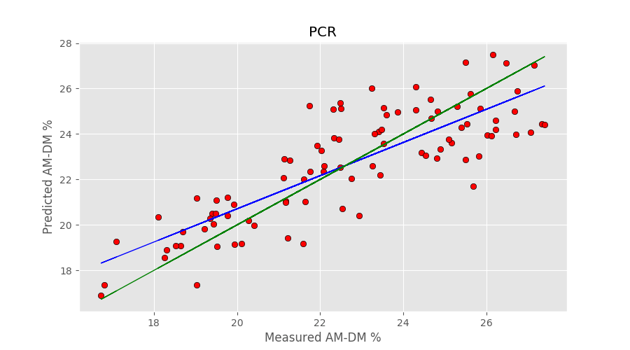
y_cv_pcr, r2r, r2cv, mser, mscv = pcr(X,y, pc=12) |
The number of principal components (12) has been optimised to get the best cross-validation result. The output of the code is
|
1 2 3 4 |
R2 calib: 0.788 R2 CV: 0.682 MSE calib: 1.647 MSE CV: 2.476 |
Now, to the Ridge Regression. Generally, the Ridge regression object is defined by calling
|
1 |
ridge = linear_model.Ridge(alpha=some_number) |
This is fine when we already know the optimal value of the hyperparameter \alpha . In general however, such a value must be evaluated by checking the cross-validation results of regressions done with different \alpha . To do this we use a handy function built for this purpose.
|
1 2 3 4 5 6 7 8 9 10 11 12 13 14 15 16 17 18 19 20 21 22 |
# Define the parameters and their range parameters = {'alpha':np.logspace(-4, -3.5, 50)} #Run a Grid search, using R^2 as the metric to optimise alpha ridge= GridSearchCV(linear_model.Ridge(), parameters, scoring='r2', cv=10) # Fit to the data ridge.fit(X, y) #Get the optimised value of alpha print('Best parameter alpha = ', ridge.best_params_['alpha']) print('R2 calibration: %5.3f' % ridge.score(X,y)) # Run a ridge regression with the optimised value ridge1 = linear_model.Ridge(alpha=ridge.best_params_['alpha']) y_cv = cross_val_predict(ridge1, X, y, cv=10) # y_cv=predicted score_cv = r2_score(y, y_cv) mse_cv = mean_squared_error(y, y_cv) print('R2 CV (Ridge): %5.3f' % score_cv) print('MSE CV (Ridge): %5.3f' % mse_cv) |
This blurb of code requires some explanation. We first run the GridSearchCV function to optimise the hyperparameter \alpha . The inputs to this function are the regression type (ridge regression for us), a dict of parameters (we just want to tweak \alpha , but you can input more), the type of scoring and the number of subdivision for cross-validation. The function then run the regression on the parameters grid specify and find the optimal cross-validation result.
As a technical detail, I first run GridSearchCV spanning a wide range of the parameter, then zoom in on the optimal region to improve the result. Once that is done, we just run a simple ridge regression with the optimal \alpha and evaluate the results. Here’s the output
|
1 2 3 4 |
Best parameter alpha = 0.000104811313415 R2 calibration: 0.804 R2 CV (Ridge): 0.661 MSE CV (Ridge): 2.642 |
 The results are quite comparable. In fairness, I haven’t done much work in optimising the results, however I just wanted to make the point of the close equivalence between ridge and PCR when it comes to NIR data. This is, in my opinion, one of the reasons why good old principal component selection methods (such as PCR or PLS) are still very much the way to go in NIR chemometrics.
Nevertheless, let’s spend a few more words on the difference between ridge and PCR, and why one may want to choose one over the other
Comparison between Principal Components Regression and Ridge Regression
Let’s venture a qualitative comparison between the two techniques. I have grouped the comparison between a few features of both regression types, which I hope will help understanding some of the fine differences between the two approaches.
| PCR | Ridge |
| Selects and keeps only the main principal components | Tunes the strength of the coefficients continuously, keeping all coefficients in play |
| The only hyperparameter is the number of principal components, which is an integer | The hyperparameter alpha can be adjusted continuously, potentially offering more flexibility |
| Great for visualisation and intuitive understanding of the data | Not so intuitive as looking for the coefficient magnitude requires some additional effort |
| Provides dimensionality reduction | Keeps the dimensionality of the problem the same |
We’ll be talking more on machine learning techniques in future posts. Until then, thanks for reading!


