
Genetic algorithms are a class of optimisation and search algorithm inspired by the mechanism of evolution by natural selection. Basic functions of a genetic algorithm (loosely) mimic the corresponding mechanisms observable in natural evolution, whereby species evolve due to the combination of random genome mutations and environmental selection.
Optimisation problems are designed to find a function that maximises (or minimises) a desired metric given the constraints of the problem. Genetic algorithms approach this problem by defining:
- A population, that is a group of potential solutions (these loosely corresponds to chromosomes).
- A fitness function, which measures the optimality of each solution according to the problem.
- Crossovers, which is the combination of two solutions, corresponding to the combination of the genetic material of two parents in an offspring)
- Random mutations that may affect individual parts of each solution.
These basic ingredients are used in an iterative fashion. Suppose that each solution (chromosome) is an array. Each element of the array is a gene. A population will be a series of arrays. A fitness function will be associated with each array so that individual arrays in the series can be ranked by it. A fraction of the ‘fittest’ arrays can be crossed over according to some rule, to form ‘offspring’ arrays. Elements (genes) of offspring arrays could undergo random mutation according to some rule. The new arrays, so formed are the starting ones for the next iteration (“generation”) of the algorithm.
In this post we present a wavelength selection algorithm based on genetic optimisation. Wavelength (or band) selection is a form of variable selection, when the variables are channels in a spectrum. This is a topic we keep coming back to, for its importance in defining chemometrics models for spectroscopy. A few examples of past posts on this topic are
- A variable selection method for PLS in Python
- Moving window PLS regression
- Wavelength band selection with simulated annealing
- Backward Variable Selection for PLS regression
The foundational ideas for variable selection methods is that not all wavelengths (or bands) in a spectrum are equally relevant to predict a quantity of interests. Variable selection methods are therefore developed to search through the large space of possibilities represented by the combination of bands that produce an optimal model.
Since it’s the first time we discuss genetic algorithms at all, we’ll start with a basic example and then move on to the actual wavelength selection algorithm.
Learning the basics with a simple example
The library of choice to develop genetic algorithms in Python is PyGAD, which is an open source, versatile package, which also works with with Keras and PyTorch (even though we won’t use this functionalities here).
We’ll be using NIR data taken from the paper In Situ Measurement of Some Soil Properties in Paddy Soil Using Visible and Near Infrared Spectroscopy by Ji Wenjun et al. The data is available here.
In this first example, we just aim at reproducing a target NIR spectrum starting from a population of random spectra, which is updated according to the rules of the genetic algorithms. First, the imports
import pandas as pd
import numpy as np
import matplotlib.pyplot as plt
import pygad
from sklearn.metrics import mean_squared_error as mse
from sys import stdout
Next, let’s load the data and select the target spectrum
# Load data and define arrays
data = pd.read_excel("File_S1.xlsx")
X = data.values[1:,8:].astype('float32')
wl = np.linspace(350, 2500, X.shape[1])
y = data["TOC"].values[1:].astype("float32")

# Pick one solution only to be the target
target_sp = X[0,:]
Next up, we need to define the fitness function. In this (admittedly contrived) example, the fitness function is a simple function of the distance between a solution and the target spectrum. As a distance metric, we pick the Mean Squared Error (MSE). Note that the convention is to define a fitness function that will have to be maximised, therefore we chose the inverse of the MSE as fitness function.
def fitness_function(ga_instance, solution, solution_idx):
    # The fitness must increase, so we take the inverse of the MSE
    fitness = 1.0 / mse(target_sp,solution)
    return fitness
Now we need to define an instance of the genetic algorithm, and here it is. Each of the argument of the function is commented, explaining its meaning.
ga_instance = pygad.GA(num_generations = 10000,
                       num_parents_mating = 10, # Number of selected solution for crossover based on their fitness
                       fitness_func = fitness_function, # Defined above
                       sol_per_pop = 50, # Solutions in a population
                       num_genes = target_sp.size, # Number of elements in each solution. Same as the shape of the target spectrum
                       init_range_low = 0.4, # Constraints the lower value each initial gene can take
                       init_range_high = 1.8,# Constraints the higher value each initial gene can take
                       mutation_percent_genes = 0.5, # Mutation rate in percent
                       mutation_type = "random", # See below
                       mutation_by_replacement = True, # This and the above specify that mutation will randomly replace one element of the array
                       random_mutation_min_val = 0.0, # Also the mutation result can be constrained with a min and max
                       random_mutation_max_val = 0.5, # See above
                       on_generation = on_gen) # Some other action to be performed in a generation can be specified here
The very last line enables us to define a function that executes at every iteration. We can choose to have an output printed to screen like this
# Print commands to be executed at each generation
def on_gen(ga_instance):
    stdout.write("\r"+str(ga_instance.generations_completed))
    stdout.write(" ")
    stdout.write(str(1.0/ga_instance.best_solution()[1]))
    stdout.flush()
All is left is to run the optimisation
ga_instance.run()
which will go through the 10,000 generations that we requested, starting from a set of random arrays (the initial solutions). At the end, we can print the best solution and compare it to the target
plt.plot(wl, target_sp, 'k', label="Target spectrum")
plt.plot(wl,ga_instance.best_solution()[0], label="GA best solution")
plt.xlabel("Wavelength (nm)")
plt.ylabel("Absorbance spectra")
plt.legend()
plt.show()
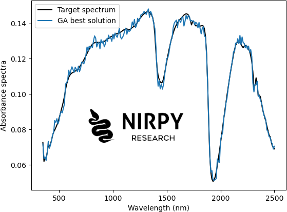
Our best solution is quite close to the target, but with some additional noise. You can play around with the parameters for instance by changing the number of solutions in a population (the more you have the better genetic diversity), the number of cross-over parents, the rate of random mutations, etc.
We can also explore how the fitness function improved as the generations progressed, using a pyGAD built-in function
ga_instance.plot_fitness()
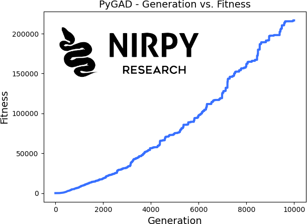
As you can realise by studying this example, all the action is in the definition of the fitness function, assuming a clever definition of the arrays and their constraints. More complicated optimisation problems, like the wavelength selection we are about to present, will have to be wrapped into the fitness function itself.
Wavelength selection
The first step to implement wavelength selection is to define a Boolean (or binary — I use the terms interchangeably here being aware of their difference in other contexts) array which specifies which bands need to be selected. If an element (i.e. a gene) of that array is True, than the corresponding band needs to be selected, otherwise neglected. So, to recap, genes are binary (True/False) and solutions are binary arrays.
Each Boolean array is the subject of the genetic optimisation. It is “evolved” through the algorithm sequence of operations aiming at maximising a fitness function.
We’ll need a few additional imports here.
from sklearn.metrics import mean_absolute_error, r2_score
from sklearn.cross_decomposition import PLSRegression
from sklearn.model_selection import cross_val_predict, GridSearchCV
Also, in order to speed up the process and make the solutions less sensitive to noise, we are going to decimate the spectra, by block-averaging every 4 consecutive wavelengths.
# Average blocks of 4 wavelengths
Xavg = X.reshape(X.shape[0], X.shape[1]//4,4).mean(axis=2)
The goal is to optimise a regression model that will predict the independent variable form the spectra. Therefore, the fitness function will have to be related to RMSE in cross-validation or similar. Following this idea, let’s first define a cross-validation (CV) function for regression. We use PLS regression here, but the same approach can be generalised to many other types of regressions
def cv_regressor(X,y, cv=5):
    # Specify parameter space
    parameters_gs = {"n_components": np.arange(8,15,1)}
    # Define Grid Search CV object
    regressor = GridSearchCV(PLSRegression(), parameters_gs, \
             cv=cv, scoring = 'neg_mean_squared_error', n_jobs=8)
    # Fit to data
    regressor.fit(X, y)
    # Calculate a final CV with best choice of parameters
    y_cv = cross_val_predict(regressor.best_estimator_, X, y, cv=5, n_jobs=8)
    return y_cv
The cv_regressor function optimises the number of latent variables and returns a prediction based on n-fold (n=5 here) CV. Now, the fitness function will have to include the cv_regressor function and calculate the fitness based on it. Here’s what you could do
def fitness_function(ga_instance, solution, solution_idx):
    # We need to explicitly set the solution array to bool
    solution = solution.astype('bool')
    # Cross-validation -- Note that X and y arrays do not need to be passed as parameters to the function!
    y_cv = cv_regressor(Xavg[:,solution], y)
    # The fitness function must increase -> take the inverse of the RMSE
    fitness = 1.0 / np.sqrt(mean_squared_error(y,y_cv.flatten()))

    return fitness
Again, keep in mind that the fitness function must increase, so we are going to take the inverse of the RMSE-CV.
In the simple example above, we had chosen to start from a completely random set of solutions in the initial population. We could do the same here of course, but I thought it could be useful to explore another possibility: define the initial population and pass it as a parameter to the GA instance. Here’s how you could generate an initial population with number of solutions per population and number of bands as parameters.
def generate_initial_population(array_size, solutions_per_pop, number_of_bands):

    # Starts with a boolean array of zeroes
    init_population = np.zeros((solutions_per_pop, array_size)).astype("bool")
    # Define an index array the size of the spectral wavelengths
    index_array = np.arange(array_size)

    for i in range(solutions_per_pop):
        # Randomly shuffle the array in place
        np.random.shuffle(index_array)
        # Select the first number_of_bands of the shuffled array and use it to flip the population array
        init_population[i, index_array[:number_of_bands]] = ~init_population[i, index_array[:number_of_bands]]

    return init_population.astype('int')
The function above lets us define the size of the initial population, and the number of bands that are initially selected (at random). Here’s how we use this function
# Here we define how many bands we want to select at the beginning
number_of_bands = 25
# This parameter define the "pool" of genetic diversity. Larger is better but slower.
solutions_per_populations = 50
# Generate the initial population
init_pop = generate_initial_population(Xavg.shape[1],
                                       solutions_per_populations,
                                       number_of_bands)
We start with 25 bands and 50 solutions per population. The GA instance is defined as
# Define the GA instance here.
ga_instance = pygad.GA(num_generations = 100,
                       num_parents_mating = 10,
                       fitness_func = fitness_function,
                       num_genes = Xavg.shape[0],
                       initial_population = init_pop, # <-- Here's the initial population definition
                       gene_type = int, # <- The genes are integer numbers. This and the next constraint ensures \
                                        # that genes can only take the values 0 or 1
                       gene_space = [0, 1], # <- The genes are constrained between zero and one.
                       mutation_percent_genes = 30,
                       mutation_type = "random",
                       on_generation = on_gen)
I tried a few different options and the one above seems to outperform the others. As you can see, we let genes undergo random mutations (i.e. each gene can randomly change from True to False independently of the other genes) with a given rate. This will not preserve the number of allowed bands, and in fact will optimise it! I found that this worked much better than the option of keeping the number of selected bands fixed.
Note that we define the genes to be integer and restricted to sit between 0 and 1. In this way we ensure that 0 and 1 are the only possible options.
We now run the instance and plot the results.
ga_instance.run()

best_solution = ga_instance.best_solution()[0].astype('bool')
y_cv_best = cv_regressor(Xavg[:,best_solution], y)  #[:,best_solution]

rmse_best, mae_best, score_best = np.sqrt(mean_squared_error(y, y_cv_best)), \
                            mean_absolute_error(y, y_cv_best), \
                            r2_score(y, y_cv_best)

print("R2: %5.3f, RMSE: %5.3f, MAE: %5.3f" %(score_best, rmse_best, mae_best))
regression_plot(y,y_cv_best, variable = "")
In fact we can also compare between the optimised solution and the original
# Comparison without optimisation
y_cv_base = cv_regressor(X, y)

rmse_base, mae_base, score_base = np.sqrt(mean_squared_error(y, y_cv_base)), \
                            mean_absolute_error(y, y_cv_base), \
                            r2_score(y, y_cv_base)

print("R2: %5.3f, RMSE: %5.3f, MAE: %5.3f" %(score_base, rmse_base, mae_base))

regression_plot(y,y_cv_base, variable = "")

In case you’re wondering, the regression_plot function was defined in this post. I’ve added the metrics at the bottom of each plot to show the improvement achieved with the genetic algorithm.
To wrap it up, the genetic optimisation has improved the metrics of the regression model by selecting bands that are better correlated to the independent variable. This was a basic example to show how the wavelength selection problem could be solved via genetic optimisation.
Well, thanks for reading until the end … and until next time!


