
Last update:
In previous posts, we have introduced Principal Components Analysis (PCA) and gave a practical example of classification. So far, however, we never really discussed the nitty-gritty of the data analysis. In this post we are going to fill that gap, and present a tutorial on how to run a classification of NIR spectra using Principal Component Analysis in Python.
PCA is nearly invariably used in the analysis of NIR data, and for a very good reason. Typical NIR spectra are acquired at many wavelengths. For instance, the data used in this post were acquired at 601 wavelength points with an interval of 2 nm. 601 data points for each spectra are, in general, a very redundant set. NIR spectra are fairly information-poor, that is they never contain sharp features, as it may be the case for Raman or MIR spectroscopy. For this reason, most of the features of NIR spectra at different wavelengths are highly correlated.
That is where PCA comes into play.
PCA is very efficient at performing dimensionality reduction in multidimensional data which display a high level of correlation. PCA will get rid of correlated components in the data by projecting the multidimensional data set (601 dimensions for this dataset) to a much lower dimensionality space, often a few, or even just two, dimensions.
These basic operations on the data are typically done using chemometrics software, and there are many excellent choices on the market. If however you would like to have some additional flexibility, for instance try out a few supervised or unsupervised learning techniques of your data, you might want to code the data analysis from scratch. This is what we are about to do in this post. Keep reading!

Reading and preparing the data for PCA analysis
We run this example using Python 3.5.2. Here’s the list of the imports we need on the first step.
|
1 2 3 4 5 6 7 8 9 |
import pandas as pd import numpy as np import matplotlib.pyplot as plt from mpl_toolkits.mplot3d import Axes3D from scipy.signal import savgol_filter from sklearn.decomposition import PCA as pca from sklearn.preprocessing import StandardScaler from sklearn import svm from sklearn.cluster import KMeans |
We are going to use NIR spectra from milk samples with a varying concentration of lactose. We prepared the samples by mixing normal milk and lactose-free milk in different concentrations.
The aim is to find out whether PCA applied to the spectra can be useful to discriminate between the different concentrations. The data is in a csv file containing 450 scans. Each scan is identified with a label (from 1 to 9) identifying the sample that was scanned. Each sample was scanned 50 times and the difference between samples was in the relative content of milk and lactose-free milk. The data is available for download at our Github repository.
|
1 2 3 4 5 6 7 8 9 10 11 12 |
# Import data from csv on github url = 'https://raw.githubusercontent.com/nevernervous78/nirpyresearch/master/data/milk.csv' data = pd.read_csv(url) # The first column of the Data Frame contains the labels lab = data.values[:,1].astype('uint8') # Read the features (scans) and transform data from reflectance to absorbance feat = np.log(1.0/(data.values[:,2:]).astype('float32')) # Calculate first derivative applying a Savitzky-Golay filter dfeat = savgol_filter(feat, 25, polyorder = 5, deriv=1) |
The last step is very important when analysing NIR spectroscopy data. Taking the first derivative of the data enables us to correct for baseline differences in the scans, and highlight the major sources of variation between the different scans. Numerical derivatives are generally unstable, so we use the smoothing filter implemented in scipy.signal import savgol_filter to smooth the derivative data out.
Picking the right number of principal components in PCA of NIR spectroscopy data
As explained before, we are going to use PCA to reduce the dimensionality of our data, that is reduce the number of features from 601 (wavelengths) to a much smaller number. So here’s the first big question: How many features do we need?
Let’s work through the answer to this question, as it may seem a bit at odd with what is usually done in some statistical analysis. Each principal component will explain some of the variation in the data. The first principal component will explain most of the variation, the second a little bit less, and so on.
To get a bit more technical, we can talk of variance explained by each principal component. The sum of variances of all principal components is called the total variance. The general advice is to choose the first n principal components that account for the large majority of the variance, typically 95% or 90% (or even 85%) depending on the problem.
This approach is not always very insightful with NIR spectroscopy data, especially when dealing with derivative data. Let’s spend some lines looking at this issue. The previous sentence may sound a bit cryptic. To explain its meaning, here’s the plot of the explained variance and the cumulative variance of the first 10 principal components extracted from our data. 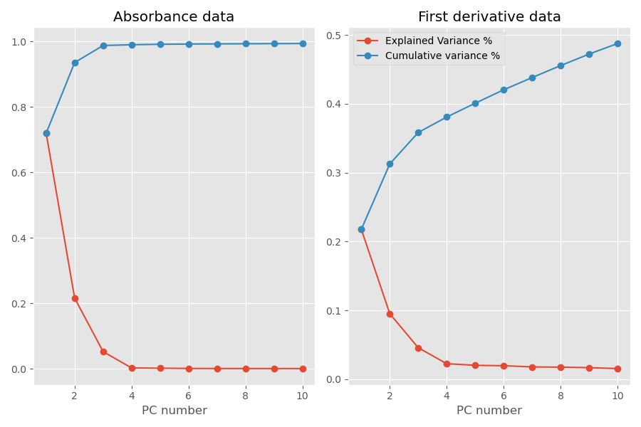 Before showing you the code we used to generate these plots, let’s take a look at the numbers. Data plotted on the left hand side refer to the PCA applied to the original absorbance data. Data on the right hand side refer to PCA applied to the first derivative data.
When applied to the original data, we see that 3 principal components account for most of the variance in the data, 98.8% to be precise. The contribution of the subsequent principal components is negligible. The situation is very different however when we run PCA on the first derivative data. Here it seems that each principal component adds a sizable bit to the variance explained, and in fact it seems that many more principal components would be required to account for most of the variance.
So, what is going on here?
I believe that the culprit is the noise present in the data. Noise is amplified in the numerical derivative operation, and that is why we need to use a smoothing filter. The filter however doesn’t get rid of the noise completely. Residual noise is uncorrelated from scan to scan, and it can’t therefore be accounted for using only a small number of principal components.
The good news is however that the most important variations in the data are in fact still described by a handful (3-4) of principal components. The higher order principal components, found when decomposing first derivative data, account mostly for noise in the data. In fact, see how the explained variance of the first derivative data flats out after 4 principal components. After that, there is negligible information in the first derivative data, just random noise variations.
So, a good rule of thumb is to choose the number of principal components by looking at the cumulative variance of the decomposed spectral data, even though we will be generally using the first derivative data for more accurate classification. OK, done with that. Here’s the code
|
1 2 3 4 5 6 7 8 9 10 11 12 13 14 15 16 17 18 19 20 21 22 23 24 25 26 27 28 29 30 31 32 33 34 35 36 |
# Initialise nc = 10 pca1 = pca(n_components=nc) pca2 = pca(n_components=nc) # Scale the features to have zero mean and standard devisation of 1 # This is important when correlating data with very different variances nfeat1 = StandardScaler().fit_transform(feat) nfeat2 = StandardScaler().fit_transform(dfeat) # Fit the spectral data and extract the explained variance ratio X1 = pca1.fit(nfeat1) expl_var_1 = X1.explained_variance_ratio_ # Fit the first data and extract the explained variance ratio X2 = pca2.fit(nfeat2) expl_var_2 = X2.explained_variance_ratio_ # Plot data pc_array = np.linspace(1,nc,nc) with plt.style.context(('ggplot')): fig, (ax1, ax2) = plt.subplots(nrows=1, ncols=2, figsize=(9,6)) fig.set_tight_layout(True) ax1.plot(pc_array, expl_var_1,'-o', label="Explained Variance %") ax1.plot(pc_array, np.cumsum(expl_var_1),'-o', label = 'Cumulative variance %') ax1.set_xlabel("PC number") ax1.set_title('Absorbance data') ax2.plot(pc_array, expl_var_2,'-o', label="Explained Variance %") ax2.plot(pc_array, np.cumsum(expl_var_2),'-o', label = 'Cumulative variance %') ax2.set_xlabel("PC number") ax2.set_title('First derivative data') plt.legend() plt.show() |
Running the Classification of NIR spectra using Principal Component Analysis in Python
OK, now is the easy part. Once we established the number of principal components to use – let’s say we go for 4 principal components – is just a matter of defining the new transform and running the fit on the first derivative data.
|
1 2 3 4 |
pca2 = pca(n_components=4) # Transform on the scaled features Xt2 = pca2.fit_transform(nfeat2) |
Finally we display the score plot of the first two principal components. You can also create a 3D scatter plot of the first 3 principal components (which we leave for another day).
|
1 2 3 4 5 6 7 8 9 10 11 12 13 14 15 16 17 18 19 20 |
# Define the labels for the plot legend labplot = ["0/8 Milk","1/8 Milk","2/8 Milk", "3/8 Milk", \ "4/8 Milk", "5/8 Milk","6/8 Milk","7/8 Milk", "8/8 Milk"] # Scatter plot unique = list(set(lab)) colors = [plt.cm.jet(float(i)/max(unique)) for i in unique] with plt.style.context(('ggplot')): plt.figure(figsize=(8,6)) for i, u in enumerate(unique): col = np.expand_dims(np.array(colors[i]), axis=0) xi = [Xt2[j,0] for j in range(len(Xt2[:,0])) if lab[j] == u] yi = [Xt2[j,1] for j in range(len(Xt2[:,1])) if lab[j] == u] plt.scatter(xi, yi, c=col, s=60, edgecolors='k',label=str(u)) plt.xlabel('PC1') plt.ylabel('PC2') plt.legend(labplot,loc='upper right') plt.title('Principal Component Analysis') plt.show() |
 That’s it for today. Thanks for reading and until next time!


