
One of the open secrets in chemometrics applied to spectroscopy is that wavelength band selection is a key ingredient. Often more important than the specific model used for multivariate calibration, band selection enables to significantly improve the quality of a prediction model.
Given the large wide wavelengths sensitivity of modern instruments, selecting the wavelength bands that better correlate with the quantity of interest is often a daunting task.
In this post we are going to use an optimisation technique called Simulated Annealing, which enables us to perform a random search in the space of possible band combinations. The aim is to find what we hope is an optimal solution.
Defining the problem of wavelength bands selection
Let’s first define what we mean by wavelength bands for the aim of this optimisation.
Most instruments nowadays have amazing spectral resolution. For many practical situations however, collinearity (also called multi-collinearity) is the norm. Collinearity refers to the fact that despite high spectral resolution, neighbouring wavelengths in many regions of the spectrum are correlated with one another. Hence, one doesn’t really need to retain all of these wavelengths for the data analysis, as adding correlated wavelengths doesn’t change the quality of the model.
As an aside, (discussed in previous posts here and here) collinearity is an actual problem for linear regression as it makes the underlying mathematical problem ill-posed. This is the reason why dimensionality reduction (via PCA or PLS for instance) is almost always required.
For the aim of this discussion, we are looking at the collinearity problem from a slightly different angle. It goes like this. If neighbouring wavelengths are correlated, we can actually average them up and in doing so producing a decimated spectrum which retains a relatively small fraction of the original wavelengths.
At this point we can easily ‘switch on/off’ individual bands (which are in fact single bins in the decimated spectrum) and check how a model will perform.
Note that this makes sense in the decimated spectrum as adding/removing bands (or swapping bands, as we’ll actually do) is likely to produce a measurable effect. Doing the same thing in the original spectrum is not likely to generate a significant difference, as many neighbouring wavelengths are equivalents.
Optimising the bands via simulated annealing
The method of simulated annealing (SA) is a clever way to produce a random optimisation. We introduced SA in a previous post already, so you can refer to that for the details.
In short, we are going to define a cost function, namely the root mean square error in cross-validation (RMSECV) and seek to decrease it. Unlike greedy algorithms which seek to monotonically decrease the cost function, SA is an optimisation process that can occasionally allow an increase of the cost function (based on some probability).
The net effect of allowing an occasional ‘worse’ solution is that the algorithm is less likely to get stuck in a local minimum. I won’t say more here. For more info you can check out my dedicated post on simulated annealing here.
Here’s the procedure we are going to follow.
- Define a number of bands we want to retain. This value, call it N, has to be obviously smaller than the total number of bands. This number is a hyper-parameter. It is fixed during the optimisation but one can try a few values out and see the result during different runs.
- Pick N random bands and start the optimisation process and fit a PLS model optimising the number of latent variables. Calculate the RMSECV as our cost function.
- At this point we start the iterative procedure. At each step we swap three bands at random and extract the RMSECV of the optimised PLS. If the new value of the RMSECV is lower than the older one, keep the swapped bands. Otherwise keep it only in accord with some small probability, driven by the cooling parameter. (Once again, for all the details of the simulated annealing optimisation, refer to my previous post).
- Repeat for a sufficient number of iterations.
At the end of the procedure we return the selected bands, alongside the optimised number of components of the PLS model associated with such a band selection. We also return a list containing the value of the RMSECV at each iteration, which we can plot to get a better understanding of how the RMSE is converging.
Here’s the entire function (for the list of imports, see next section).
|
1 2 3 4 5 6 7 8 9 10 11 12 13 14 15 16 17 18 19 20 21 22 23 24 25 26 27 28 29 30 31 32 33 34 35 36 37 38 39 40 41 42 43 44 45 46 47 48 49 50 51 52 53 54 55 56 57 58 59 60 61 62 63 64 65 66 67 68 69 70 |
def band_selection_sa(X,y,n_of_bands, max_lv, n_iter): p = np.arange(X.shape[1]) np.random.shuffle(p) bands = p[:n_of_bands] # Selected Bands. Start off with a random selection nbands = p[n_of_bands:] # Excluded bands Xop = X[:,bands] #This is the array to be optimised # Run a PLS optimising the number of latent variables opt_comp, rmsecv_min = pls_optimise_components(Xop, y, max_lv) rms = [] # Here we store the RMSE value as the optimisation progresses for i in range(n_iter): cool = 0.001*rmsecv_min # cooling parameter. It decreases with the RMSE new_bands = np.copy(bands) new_nbands = np.copy(nbands) # swap three elements at random for jj in range(3): r1, r2 = np.random.randint(n_of_bands),np.random.randint(X.shape[1]-n_of_bands) el1, el2 = new_bands[r1],new_nbands[r2] new_bands[r1] = el2 new_nbands[r2] = el1 Xop = X[:,new_bands] opt_comp_new, rmsecv_min_new = pls_optimise_components(Xop, y, max_lv) # If the new RMSE is less than the previous, accept the change if (rmsecv_min_new < rmsecv_min): bands = new_bands nbands = new_nbands opt_comp = opt_comp_new rmsecv_min = rmsecv_min_new rms.append(rmsecv_min_new) stdout.write("\r"+str(i)) stdout.write(" ") stdout.write(str(opt_comp_new)) stdout.write(" ") stdout.write(str(rmsecv_min_new)) stdout.flush() # If the new RMSE is larger than the previous, accept it with some probability # dictated by the cooling parameter if (rmsecv_min_new > rmsecv_min): prob = np.exp(-(rmsecv_min_new - rmsecv_min)/cool) # probability if (np.random.random() < prob): bands = new_bands nbands = new_nbands opt_comp = opt_comp_new rmsecv_min = rmsecv_min_new rms.append(rmsecv_min_new) stdout.write("\r"+str(i)) stdout.write(" ") stdout.write(str(opt_comp_new)) stdout.write(" ") stdout.write(str(rmsecv_min_new)) stdout.flush() else: rms.append(rmsecv_min) stdout.write("\n") print(np.sort(bands)) print('end') return(bands, opt_comp,rms) |
Result: bands optimisation for Brix prediction in fresh plums
It’s now time to check how this band optimisation works with real data.
We are going to use NIR spectra of fresh plums and we are trying to predict the sugar content (measured in degree Brix) from the spectra.
In the following we are going to write the main part of the script. The code of all functions is copied at the end of the post and the entire Jupyter Notebook is available on Github. Let’s start with the imports.
|
1 2 3 4 5 6 7 8 9 10 11 12 |
import numpy as np import matplotlib.pyplot as plt import matplotlib.collections as collections import pandas as pd from scipy import interpolate from scipy.signal import savgol_filter from sys import stdout from sklearn.cross_decomposition import PLSRegression from sklearn.metrics import mean_squared_error, r2_score from sklearn.model_selection import cross_val_predict |
Now let’s import and preprocess the data. The Multiplicative Scatter Correction function used here is copied at the end of the post and discussed here.
|
1 2 3 4 5 6 7 8 9 10 11 12 13 14 15 16 17 18 19 20 |
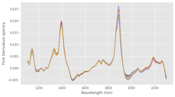
# Load data from Nirpy Reserach Github data page url = "https://raw.githubusercontent.com/nevernervous78/nirpyresearch/master/data/NIRplums_brix_firmness.csv" data = pd.read_csv(url) wl = np.linspace(1102, 2300, 600) # Extract the arrays X = -np.log(data.values[:,3:]) brix = data["Brix"] # Multiplicative Scatter Correction Xc, ref = msc(X) # First Derivative Smoothing Xc = savgol_filter(Xc,11,3, deriv=1) # Plot Data with plt.style.context(('ggplot')): fig, ax = plt.subplots(figsize=(9, 5)) ax.plot(wl, Xc.T) ax.set_xlabel("Wavelength (nm)") ax.set_ylabel("First Derivative spectra") plt.show() |
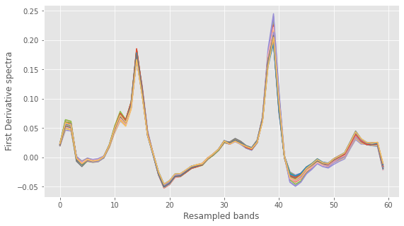
Now we are going to resample the wavelengths into bands. Since we have 600 wavelengths, let’s decimate it by a factor of 10, down to 60 bands.
|
1 2 3 4 5 6 7 8 9 |
# Resample spectra. Here is 60 bands XX = Xc.reshape(Xc.shape[0],60,10).sum(axis=2) with plt.style.context(('ggplot')): fig, ax = plt.subplots(figsize=(9, 5)) ax.plot(XX.T) ax.set_xlabel("Resampled bands") ax.set_ylabel("First Derivative spectra") plt.show() |
Before we begin the band selection algorithm, let’s check a basic PLS regression against which we’ll benchmark the optimised results. The three functions called here are defined at the end of the post. The first function will optimise the PLS components. The second runs a PLS regression with the optimal number of components. Finally the third function is just a utility function to plot the results.
|
1 2 3 4 5 6 7 |
opt_comp, rmsecv_min = pls_optimise_components(Xc, brix, 20) predicted, r2cv, rmscv = base_pls(Xc, brix, opt_comp) print("PLS results:") print(" R2: %5.3f, RMSE: %5.3f"%(r2cv, rmscv)) print(" Number of Latent Variables: "+str(opt_comp)) regression_plot(brix, predicted, title="Basic PLS", variable = "Brix") |
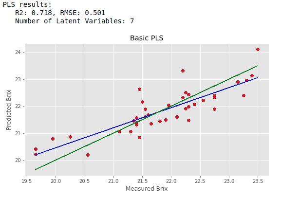
The result is OK, but not great.
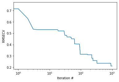
It’s time to run the Simulated Annealing algorithm and see if we can get any better. We choose 20 bands, a maximum of 20 latent variables for the PLS search and a total of 100 iterations. After the algorithm has finished we run a basic PLS with the selected bands and number of components, and we plot the results.
|
1 2 3 4 5 6 7 8 |
bands, opt_comp, rms = band_selection_sa(XX,brix,n_of_bands = 20, max_lv = 20, n_iter = 1000) predicted, r2cv, rmscv = base_pls(XX[:,bands], brix, opt_comp) print("PLS optimised bands:") print(" R2: %5.3f, RMSE: %5.3f"%(r2cv, rmscv)) print(" Number of Latent Variables: "+str(opt_comp)) regression_plot(brix, predicted, title="Optimised Bands", variable = "Brix") |
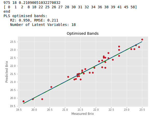
The result is way better than the basic PLS above. The algorithm has halved the RMSECV with a massive improvement in the coefficient of determination. Note that the result of each individual run of the Simulated Annealing code may vary due to the randomness of the process. We expect however that the final results will differ little from one another. If that is not happening it is likely that the model is overfitting the data.
To gain some insights into the progress of the optimisation, we can plot the rms
|
1 2 3 4 |
plt.semilogx(rms) plt.xlabel("Iteration #") plt.ylabel("RMSECV") plt.show() |
Also, we can take a look a which bands the algorithm has selected. Here’s the code to do that.
|
1 2 3 4 5 6 7 8 9 10 11 12 13 14 15 |
# ix is the index of the selected bands ix = np.in1d(np.arange(60).ravel(), np.sort(bands)) # To overlap the bands on the original spectrum, we restore the original band size ixx = np.repeat(ix,10) # Plot spectra with superimposed selected bands with plt.style.context(('ggplot')): fig, ax = plt.subplots(figsize=(9,5)) ax.plot(np.arange(Xc.shape[1]),Xc.T) plt.ylabel('First derivative spectra') plt.xlabel('Original wavelength bins') collection = collections.BrokenBarHCollection.span_where( np.arange(Xc.shape[1]), ymin=-1, ymax=1, where=(ixx == True), facecolor='green', alpha=0.3) ax.add_collection(collection) plt.show() |
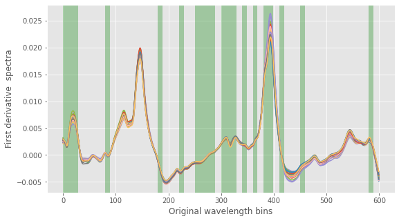
By running the code a few times, we can easily check that most of the bands are selected each time (which is related to the stability of the solution during multiple runs we have hinted at before).
That’s us for now. Thanks for reading and until next time,
Daniel
Reference of the Python functions used in this post
|
1 2 3 4 5 6 7 8 9 10 11 12 13 14 15 16 17 18 19 20 21 22 23 |
def msc(input_data, reference=None): ''' Perform Multiplicative scatter correction''' # mean centre correction for i in range(input_data.shape[0]): input_data[i,:] -= input_data[i,:].mean() # Get the reference spectrum. If not given, estimate it from the mean if reference is None: # Calculate mean ref = np.mean(input_data, axis=0) else: ref = reference # Define a new array and populate it with the corrected data data_msc = np.zeros_like(input_data) for i in range(input_data.shape[0]): # Run regression fit = np.polyfit(ref, input_data[i,:], 1, full=True) # Apply correction data_msc[i,:] = (input_data[i,:] - fit[0][1]) / fit[0][0] return (data_msc, ref) |
|
1 2 3 4 5 6 7 8 9 10 11 12 13 14 15 16 17 |
def base_pls(X,y,n_components, return_model=False): # Simple PLS pls_simple = PLSRegression(n_components=n_components) # Fit pls_simple.fit(X, y) # Cross-validation y_cv = cross_val_predict(pls_simple, X, y, cv=10) # Calculate scores score = r2_score(y, y_cv) rmsecv = np.sqrt(mean_squared_error(y, y_cv)) if return_model == False: return(y_cv, score, rmsecv) else: return(y_cv, score, rmsecv, pls_simple) |
|
1 2 3 4 5 6 7 8 9 10 11 12 13 14 15 16 17 18 19 20 |
def pls_optimise_components(X, y, npc): rmsecv = np.zeros(npc) for i in range(1,npc+1,1): # Simple PLS pls_simple = PLSRegression(n_components=i) # Fit pls_simple.fit(X, y) # Cross-validation y_cv = cross_val_predict(pls_simple, X, y, cv=10) # Calculate scores score = r2_score(y, y_cv) rmsecv[i-1] = np.sqrt(mean_squared_error(y, y_cv)) # Find the minimum of ther RMSE and its location opt_comp, rmsecv_min = np.argmin(rmsecv), rmsecv[np.argmin(rmsecv)] return (opt_comp+1, rmsecv_min) |
|
1 2 3 4 5 6 7 8 9 10 11 12 13 14 15 16 17 |
def regression_plot(y_ref, y_pred, title = None, variable = None): # Regression plot z = np.polyfit(y_ref, y_pred, 1) with plt.style.context(('ggplot')): fig, ax = plt.subplots(figsize=(9, 5)) ax.scatter(y_ref, y_pred, c='red', edgecolors='k') ax.plot(y_ref, z[1]+z[0]*y_ref, c='blue', linewidth=1) ax.plot(y_ref, y_ref, color='green', linewidth=1) if title is not None: plt.title(title) if variable is not None: plt.xlabel('Measured ' + variable) plt.ylabel('Predicted ' + variable) plt.show() |


