Principal Component Regression in Python

Hi everyone, and welcome to our easy introduction to Principal Component Regression in Python!

Principal Component Regression (PCR, in brief)  is the natural extension of Principal Components Analysis (PCA) when it comes to regression problems. We discussed PCA in our previous posts. We explained how PCA is great for clustering and classification of NIR or other spectroscopic data. A fairly extensive introduction on using PCA for NIR data in Python is in here. Feel free to check out some of our related posts:

• PCR vs Ridge Regression
• PCA classification of NIR spectra

PCA is extremely valuable for classification, as it allows us to reduce the number of variables that are effectively used to describe the data. Typical NIR spectra are acquired at many wavelengths. For instance, with our Luminar 5030 we typically acquire 601 wavelength points with an interval of 2 nm.

That means each scan will contain 601 variables. When we want to relate a NIR scan with a specific chemical or physical parameter of our sample, we generally do not need these many variables. Often just a handful of independent variables are sufficient to describe the action of the parameter of interest on our spectrum. I know, I know, that is getting confusing. To make things easier we are going to work on a specific example. We are going to discuss a basic way of building a NIR calibration for Brix in fresh peaches using NIR data. Brix, or more precisely degree Brix (°Bx), is the measure of the sugar content in a solution. For fresh fruit Brix gives a measure of the sugars in it, which is an important parameter to establish the eating quality of the fruit, and therefore its market value.

Principal Component Regression for NIR calibration

Let’s go back to our basic explanation of PCA and PCR using a specific example. We want to build a calibration for Brix using NIR spectra from 50 fresh peaches. As mentioned before, each spectrum is composed of 601 data points. To build the calibration we are going to correlate somehow the spectrum of each peach (no pun intended!) with its value of Brix measured independently with another method. As you can see already, we are going to reduce 601 data points to a single parameter! That means in practice one never needs this many points. Just a few would be sufficient.

But which variables are the one that are significant to describe Brix variation? Well, we don’t know that in advance, and that is why we are going to use PCA to sort things out. PCA is going to reduce the dimensionality of our data space, getting rid of all the variables (data points) that are highly correlated with one another. In practice we will reduce 601 dimensions (the measured wavelengths) to a much lower number, often a few, or even just two, dimensions.

This is really great, and you can check out our previous post for the nuts and bolts on how to do that in Python. With PCA we can establish that different pieces of fruit may have different Brix values, but we won’t be able to build a model that is able to predict Brix values from future measurements. The reason is that PCA makes no use whatsoever of the additional information we may have, namely the independent data of Brix measured with a different instrument. In order to use the additional information we need to go from a classification problem to a regression problem. Enters PCR.

Python implementation of Principal Component Regression

To put is very simply, PCR is a two-step process:

1. Run PCA on our data to decompose the independent variables into the ‘principal components’, corresponding to removing correlated components
2. Select a subset of the principal components and run a regression against the calibration values

Easy as pie.

Well, yes, but a word of warning is called for. In the apparent simplicity of PCR lies also its main limitation. Using PCA to extract the principal components in step 1 is done disregarding whichever information we may have on the calibration values. As noted by Jonathon Shlens in his superb paper on PCA (available here), PCA is a ‘plug&play’ technique. It spits out some results regardless of the nature of the input data, or its underlying statistics. In other words, PCA is very simple, but sometimes may be wrong.

These limitations are inherited by PCR, in the sense that the principal components found by PCA may not be the optimal ones for the regression we want to run. This problem is alleviated by Partial Least Square Regression (PLS) which we will discuss in the future. For the moment, let’s leverage the simplicity of PCR to understand the basics of the regression problem, and hopefully enjoy building the same simple calibration model of our own in Python.

OK, let’s write some code. We run this tutorial on Python 3.5.2. Here’s the list of imports.

Now let’s load the data and take a look at it. The data is available for download at our Github repository.

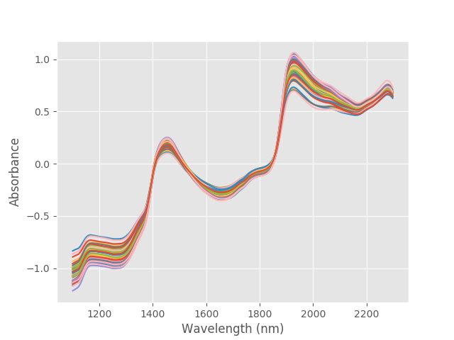These are the absorbance spectra of our 50 samples. As mentioned, we divide the PCR problem in two steps. The first is to run PCA on the input data. Before that, we have two preprocessing steps. The first is quite common in NIR spectroscopy: take the first derivative of the absorbance data Check out our previous post for more details. The second is a staple of PCA: standardise the features to subtract the mean and reduce to unit variance.

Note that in the last step, after running PCA, only the first pccomponents were selected. This will be clear in a bit, when we’ll put the whole thing in a standalone function. And now the juicy part, step by step.

We first created the linear regression object and then used it to run the fit. At this point the savvy practitioner will distinguish between calibration and cross-validation results. This is an important point, and we’ll make a short digression to cover it.

Calibration and cross-validation

In the example above, we build a linear regression between the variables Xregand y. Loosely speaking we build a linear relation between principal components extracted from spectroscopic data and the corresponding Brix values of each sample. So we expect that, if we have done a good job, we should be able to predict the value of Brix in other samples not included in our calibration.

First, how do we know if we’ve done a good job? The metrics we use are the coefficient of determination (or R^{2}) and the mean squared error (MSE). The ideas goes like this. With the regr.fit(Xreg, y) command we generate the coefficients of the linear fit (slope m and intercept q). With the y_c = regr.predict(Xreg)command we can then use these coefficients to ‘predict’ the new values y_{c} = mX_{reg}+q of the Brix given the input spectroscopy data. R^{2} tells us how well y_{c} correlates with y (Ideally we want R^{2} to be as close as possible to 1). MSE is the mean squared deviation of the y_{c} with respect to the y in the units of y, so in our case MSE will be measured in °Bx.

OK, here’s the issue. If we take the same data used for the fit and use it again for the prediction, we run the risk of reproducing our calibration set magnificently, but not being able to predict any future measurement. This is what data scientists call overfitting. Overfitting means we built a model that perfectly describes our input data, but just that and nothing else.

In order to make predictions we want to be able to handle future (unknown) data with good accuracy. For that, we would ideally need an independent set of spectroscopy data, often referred to as validation data. If we do not have an independent validation set, the next best thing is to split our input data into calibration and cross-validation sets. Only the calibration data are used to build the regression model. The cross-validation data are then used as a (hopefully) independent set to verify the predictive value of our model. Scikit-learn comes with a handy function to do just that: y_cv = cross_val_predict(regr, Xreg, y, cv=10). The parameter cv=10 means that we divide the data in 10 parts and hold out one part for cross validation.

Needless to say that we want to quantify the predictive power of our model by monitoring the metrics for the cross validation set.

Building the calibration model

To make life a bit easier for you, we have collected all the bits of code above into a handy function.

Now, to build your calibration model, all you have to do is to run the function above with a variable number of principal components, and decide which value gives the best results. For instance, if we test the calibration for up to 20 principal components, that’s what we get: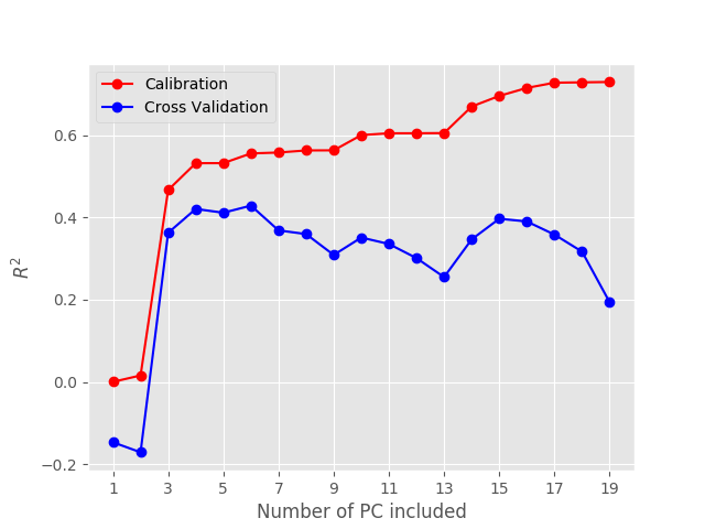

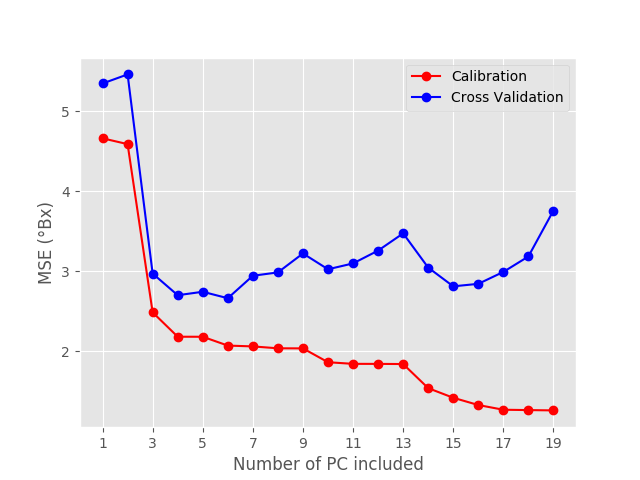Both R^{2} and MSE have a sudden jump at the third principal component, which indicates that 3 principal components are required, at the very least, to describe the data.

As expected, the calibration metrics get better and better the more principal components we add. However, what’s important for us are the cross validation values. Specifically we are going to look for a minimum in the MSE, which occurs for PC=6. If we add more principal components, the cross validation MSE gets actually worse. That is six the optimal number of principal components to pick.

With the knowledge of the optimal value, we are ready to plot the actual prediction.

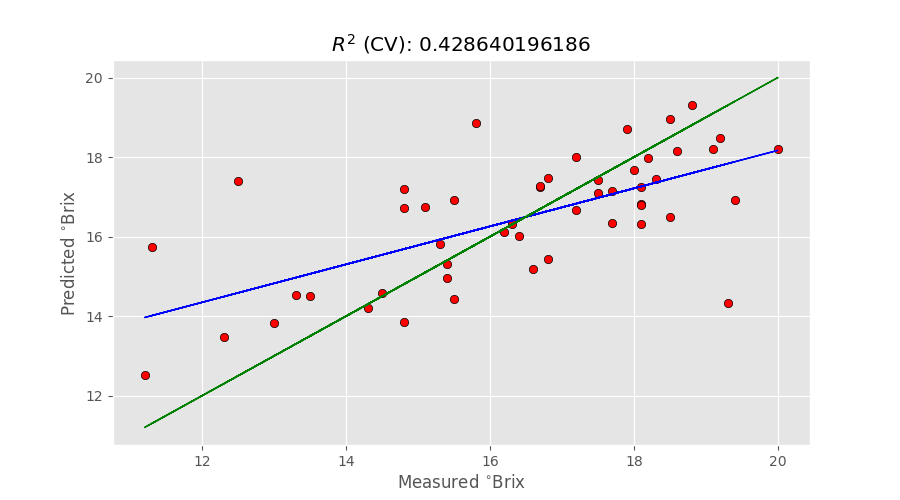The green line represents the ideal, 100%, correlation between measured and predicted values. The blue line is the actual correlation.  With R^{2}=0.43 the result is obviously not great, and a number of other things are required to improve this figure. Things about multiplicative scatter correction and feature selection are often used to improve the prediction. At the same time, the main limitation of the PCR approach (the fact the PCA is done without knowledge of the y values) also plays a big role in the final results.

Typically, better results can be obtained with Partial Least Squares (PLS), which is another of our posts you should check out.

Optimising the model with scikit-learn built-in functions

Now that we learnt the basics of PCR, we can look at a shortcut to optimise a PCR model usingscikit-learn built-in functions, namely Pipeline and GridSearchCV. Pipeline allows us to chain two or more transformations in a single estimator. For PCR we need to combine PCA and Linear Regression.

As we just learnt, optimising a PCR model means finding the number of principal components that minimises the RMSE in cross-validation. GridSearchCV can be used for that (and many other things). All we need to do is to define one or more parameters to be optimised, and the range over which we want to sweep them. In our case a single parameter is needed.

Here’s the code, including the imports

Conveniently, GridSearchCV optimisation is done by fitting it to the dataset. The pcr._best_estimator_ is then the optimal model, so that it can be again fitted to the data so

That’s it for today and I hope you enjoyed this post. Thanks for reading!