
In one of our first posts on the NIR regression series, we discussed the basics of Principal Components Regression (PCR). Here we are going to revisit the concept of PCR, and discuss a clever hack that will help you significantly improve the quality of the model.
PCR is the combination of Principal Components Analysis (PCA) decomposition with linear regression. When dealing with highly collinear data, such as NIR spectra, it would be foolish to set up a linear regression with the spectral data of individual bands, as there is a high level of correlation (collinearity) between neighbouring bands.
A more clever way to work with this kind of data is to decompose the data in a way that reduce the collinearity problem, and distil the best possible information out of the original data. PCA is one such decomposition. Principal components represent a decomposition of the original data into orthogonal directions. In this way the collinearity problem is removed (orthogonal means there is no correlation between each individual components) while all the information present in the original data is preserved.
Principal components are sorted in order of explained variance. The first component is the one that explain the most of the variance of the data, followed by the second and so on. Usually the last (least important) components tend to relate to noise that is naturally present in the data. For more details on PCA and PCR you can take a look at our previous posts.
Principal Component Regression
Let’s quickly recap the main concepts of PCR. The gist of PCR is establishing a linear regression model using but a few principal components. Following the fact that the first few principal components explain most of the variance in the data, one could select only these and use them as independent variable in the regression problem. In this way we solve the collinearity problem (the principal components are uncorrelated to one another) and retain most of the variability in our original dataset.
In our first post on PCR we explained how to select the number of principal components to use. We use the mean squared error (MSE) in cross-validation as the metric to minimise. That is we run a PCR with an increasing number of principal components and check which number yields the minimum MSE.
Here’s a recap of how we can do this in Python. Let’s begin with the imports
|
1 2 3 4 5 6 7 8 9 |
import pandas as pd import numpy as np import matplotlib.pyplot as plt from sklearn.decomposition import PCA from sklearn.preprocessing import StandardScaler from sklearn import linear_model from sklearn.model_selection import cross_val_predict from sklearn.metrics import mean_squared_error, r2_score |
Now let’s define a function that performs a simple linear regression on input data and runs a cross-validation procedure to estimate coefficient of determination (in Python called “score”) and the MSE.
|
1 2 3 4 5 6 7 8 9 10 11 12 13 14 15 16 17 18 19 20 21 22 23 |
def simple_regression(X,y): # Create linear regression object regr = linear_model.LinearRegression() # Fit regr.fit(X, y) # Calibration y_c = regr.predict(X) # Cross-validation y_cv = cross_val_predict(regr, X, y, cv=10) # Calculate scores for calibration and cross-validation score_c = r2_score(y, y_c) score_cv = r2_score(y, y_cv) # Calculate mean square error for calibration and cross validation mse_c = mean_squared_error(y, y_c) mse_cv = mean_squared_error(y, y_cv) return(y_cv, score_c, score_cv, mse_c, mse_cv) |
Finally, we define a PCR function, which first runs a PCA decomposition and then linear regression on the input data.
|
1 2 3 4 5 6 7 8 9 10 11 12 13 14 15 16 17 18 19 |
def pcr(X,y, pc): ''' Step 1: PCA on input data''' # Define the PCA object pca = PCA() # Preprocess (2) Standardize features by removing the mean and scaling to unit variance Xstd = StandardScaler().fit_transform(X) # Run PCA producing the reduced variable Xred and select the first pc components Xreg = pca.fit_transform(Xstd)[:,:pc] ''' Step 2: regression on selected principal components''' y_cv, score_c, score_cv, mse_c, mse_cv = simple_regression(Xreg, y) return(y_cv, score_c, score_cv, mse_c, mse_cv) |
Note that the PCR function above requires an additional argument which we called pc. That is the maximum number of principal components to be selected. The PCA operation yields as many components as spectra or wavelengths (depending on whichever is largest) but we do not need them all for the regression. Better still, we must select only a few components to have a chance of getting a good model, as the highest order components tend to be noisier and reduce the quality of the model.
Since we do not know the optimal value of pc for our problem, we are going to run this function in a loop and minimise the MSE. The data is available for download at our Github repository.
|
1 2 3 4 5 6 7 8 9 10 11 12 13 14 15 |
# Read data: NIR spectra of peaches with corresponding Brix calibration data data = pd.read_csv('./data/peach_spectra+brixvalues.csv') X = data.values[:,1:] y = data['Brix'] npc = 40 # maximum number of principal components pc = range(1,npc+1,1) # Define arrays for R^2 and MSE r2c = np.zeros(npc) r2cv = np.zeros(npc) msec = np.zeros(npc) msecv = np.zeros(npc) for i in pc: predicted, r2c[i-1], r2cv[i-1], msec[i-1], msecv[i-1] = pcr(X,y, pc=i) |
At the end of the run we plot the MSE arrays for both calibration and cross validation (CV). What we’re after is the minimum for RMSE-CV which is the root mean squared error (i.e. the square root of MSE).
|
1 2 3 4 5 6 7 8 |
with plt.style.context(('ggplot')): plt.plot(pc, np.sqrt(msecv[:]), 'r', label = "RMSECV") plt.plot(pc, np.sqrt(msec[:]), 'b', label = "RMSEC") plt.xlabel("# Principal Components") plt.ylabel("RMSE") plt.title("Conventional PCR") plt.legend() plt.show() |
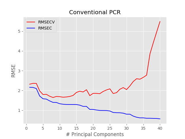
The minimum RMSE occurs for pc = 8. Therefore we can run the pcr function with such value and plot the regression results.
|
1 2 3 4 5 6 7 8 9 10 11 12 |
predicted, r2r, r2cv, mser, mscv = pcr(X,y, pc=8) # Regression plot z = np.polyfit(y, predicted, 1) with plt.style.context(('ggplot')): fig, ax = plt.subplots(figsize=(9, 5)) ax.scatter(y, predicted, c='red', edgecolors='k') ax.plot(y, z[1]+z[0]*y, c='blue', linewidth=1) ax.plot(y, y, color='green', linewidth=1) plt.title('Conventional PCR -- $R^2$ (CV): {0:.2f}'.format(r2cv)) plt.xlabel('Measured $^{\circ}$Brix') plt.ylabel('Predicted $^{\circ}$Brix') plt.show() |

Here we go, this is the result. Not great we must admit.
The reason is a fundamental problem with the procedure. PCA decomposition is an unsupervised learning method. In a machine learning language, PCA decomposition maximises the explained variance in the data without accounting for any labels (calibration values). In NIR regression problems, if we have a primary calibration value (in our example would be the Brix in fresh peaches) the directions that explain most of the variance of the spectra are not necessarily those that better explains the changes in Brix.
Thus, there is no guarantee that the first 8 principal components we selected are the ones that better correlates with changes in Brix. To be clear, there is a likelihood that the first principal components are also partly correlated with the variation of interest (the regression plot above is not flat after all), but that is by no mean given as far as the algebra of the problem is involved. In other words, PCA looks only at the spectra and not at the calibration values.
Partial Least Squares (PLS) is a way to solve this problem, as PLS accounts for the calibration values as well. The simplicity of PCR however is very attractive and I’m going to show you how, with a simple hack, we can re-introduce some knowledge of the calibration values (labels) into the PCR framework.
Principal Component Regression in Python revisited
OK, so in our previous post we simply selected an increasing number of principal components and check the resulting regression metric. The order in which these components were sorted was the one that naturally arises from a PCA decomposition, that is following explained variance.
Here’s a simple idea. Why not to check the correlation between each principal component and the calibration values? In this way we could sort the principal components in order of increasing (or decreasing) correlation and use this new ordering to maximise the regression metrics.
Note that, by doing this, we are putting back some information on the labels from the back door. The principal components are what they are. They are defined by the explained variance. The principal components we decide to pick however are the one that better correlate with the feature of interest.
Here is how we go about doing that in Python.
|
1 2 3 4 5 6 7 8 9 10 11 12 13 14 15 16 17 18 19 20 21 22 23 24 25 26 |
def pcr_revisited(X,y, pc): ''' Step 1: PCA on input data''' # Define the PCA object pca = PCA() # Preprocess (2) Standardize features by removing the mean and scaling to unit variance Xstd = StandardScaler().fit_transform(X) # Run PCA producing the reduced variable Xreg and select the first pc components Xpca = pca.fit_transform(Xstd) # Define a correlation array corr = np.zeros(Xpca.shape[1]) # Calculate the absolute value of the correlation coefficients for each PC for i in range(Xpca.shape[1]): corr[i] = np.abs(np.corrcoef(Xpca[:,i], y)[0, 1]) # Sort the array based on the corr values and select the last pc values Xreg = (Xpca[:,np.argsort(corr)])[:,-pc:] ''' Step 2: regression on selected principal components''' y_cv, score_c, score_cv, mse_c, mse_cv = simple_regression(Xreg, y) return(y_cv, score_c, score_cv, mse_c, mse_cv) |
The hack we are talking about happens at lines 14-21 of the snippet above. In words,
- We calculate the correlation coefficient of each PC array with the calibration values
- We take the absolute value, as positive or negative correlations are equally good for our purpose. What we want to reject are the PC that have correlation values close to zero.
- We sort the PC array in order of increasing correlation.
- We select the last pc values of the array, as they are the ones with the largest correlation
Once we have done that, we run the linear regression, just as before. The result however is going to be extremely different: here’s the RMSE plot that we get using the new function in the for loop
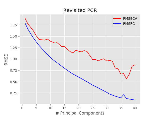
Two important differences are visible. The first is that the minimum occurs at a much larger value of pc, 37 in this case. The second is that the minimum RMSE is less than half of what it was before. That means that the model we are generating now is a much better fit to the data.
And in fact, here’s the regression plot

The difference is remarkable. We get R^{2}= 0.93 in cross-validation. And all we have done is to rearrange the principal components depending on the level of correlation they have with the calibration data
Wrap up and a few comments
Lets’ recap the main points of this post.
- PCR is a straightforward regression technique. Very easy to optimise and interpret
- A major drawback of PCR is that the calibration values are not accounted for during the PCA decomposition
- We can partially account for the calibration values by calculating the correlation coefficients of each principal components with the calibration values. We can use this information to sort the PCA array in an optimal way
- The comparison between simple PCR and revisited PCR is stunning: we get a way better model using this simple hack. However, given the small number of data points, one needs to be very careful about how such a model can generalise. The important thing to check is how the selected principal components are representative of the original dataset.
Three final comments.
The revisited PCR techniques uses more principal components, 37 versus 8 in this example to achieve a much better result. This clearly means that 8 components are obviously not enough to describe the variability of our data with respect to Brix. However, since the magnitude of each subsequent PC is reduced, we can’t select the best values just by running through the original PCA array. The hack of reordering the PCA array enables that.
Since we are sorting the PC in order of increasing correlation, it follows that the specific sorting will be different for different features. For instance we could decide to build a regression model for Brix and flesh firmness from our NIR data and we would expect the principal components would be sorted differently in each model.
It is very important to check that the PC selected as better correlated to the labels, are in fact representative of real features and not noise. In other words, this model is very prone to overfitting if caution is not exercised. I’ve shown here the model on a relatively small dataset to give an idea of the code in a way that is easy to test out. I would not expect however, in this example, that the model will be robust. By greatly increasing the training set, and possibly reducing the total number of PC under consideration, this hack may be a good tool in your statistical learning toolbox.
Hope you enjoyed reading this post. If you found it useful, please share it with a colleague, it will help us grow. Thanks for reading!


