Cross-Validation (CV) is a standard procedure to quantify the robustness of a regression model. The basic idea of CV is to test the predictive ability of a model on a set of data that has not been used to build that model. K-fold cross-validation is probably the most popular amongst the CV strategies, however other choices exist. In this tutorial we are going to look at three different strategies, namely K-fold CV, Montecarlo CV and Bootstrap. We will outline the differences between those methods and apply them with real data.
A few references that may be useful for working through this post are:
- Cross-Validation Wikipedia entry
- Tutorial on cross-validation from scikit-kearn
- Bootstrap aggregating entry on Wikipedia
Before delving into the details, a short note on terminology. While K-Fold is a standard term for the associated algorithm, both Montecarlo and Bootstrap are often found under different names. Montecarlo CV is also called Shuffle Split or Random Permutation CV. Bootstrap (or bootstrapping) in machine learning is more correctly called Bootstrap Aggregating, or (shortened to) Bagging. Regardless of the terminology, we are going to define exactly what we mean by each method, so to avoid confusion when comparing different sources. I also must say that Bootstrap is not, strictly speaking, a cross-validation method (we will clarify this later), but we are going to use it in a similar fashion as the other two methods.
The data used in this articles are taken from the paper Near‐infrared spectroscopy (NIRS) predicts non‐structural carbohydrate concentrations in different tissue types of a broad range of tree species, by J. A. Ramirez et al. The associated dataset is freely available for download here.
K-fold, Montecarlo and Bootstrap
To quantify the robustness of a regression model with a single dataset — i.e. without an independent test set — requires splitting the available data into two or more subsets, so that model fitting and prediction can be performed on independent subsets. This typical strategy can be implemented in various ways, all aimed at avoiding overfitting. Overfitting refers to the situation in which the regression model is able to predict the training set with high accuracy, but does a terrible job at predicting new, independent, data. In other words, the model is mostly built on features that are specific to training set, with can bear little correlation with new data. A cross-validation strategy avoids or mitigates this occurrence.
In this section we are going to define K-fold, Montecarlo and Bootstrap using Scikit-learn in Python and describe their action on a simple array. In the next section we are going to discuss the comparison between the methods.
Let’s begin with the imports (some of which will be used later).
|
1 2 3 4 5 6 7 8 9 |
import numpy as np import matplotlib.pyplot as plt import pandas as pd from sys import stdout from sklearn.model_selection import KFold, ShuffleSplit, train_test_split from sklearn.utils import resample, check_random_state from sklearn.cross_decomposition import PLSRegression from sklearn.metrics import mean_squared_error, r2_score |
Let’s now define a simple array, of just 10 elements:
|
1 |
ar = np.array([0,1,2,3,4,5,6,7,8,9]) |
We are going to apply the different methods on this simple array, which makes it easier to check the action of the different operations. Let’s start with the K-Fold.
|
1 2 3 4 5 6 7 |
# K-Fold cross-validation split kf = KFold(n_splits=3, shuffle=True, random_state=1) # Returns the number of splitting iterations in the cross-validator kf.get_n_splits(ar) for train, test in kf.split(ar): print("Train:", ar[train]," Test:", ar[test]) |
The class Kfold is defined by passing the number of splits (“folds”) which we are going to divide our array into, the “shuffle” keywords that indicates whether we want a random permutation of the entries before splitting, and the (optional) random state for reproducibility.
After returning the number of splitting iterations, the method kf.split(ar) produces what in Python is called a generator, that is a function that can be used like an iterator in a loop. In this case the function yields the indices that split the original array into train and test set. Since we have defined three splits, this procedure is going to be repeated three times, with (approximately) a third of the data reserved for the test set. If you ruin the previous snippet you get:
|
1 2 3 |
Train: [0 1 3 5 7 8] Test: [2 4 6 9] Train: [2 4 5 6 7 8 9] Test: [0 1 3] Train: [0 1 2 3 4 6 9] Test: [5 7 8] |
The main feature of the K-Fold approach is that each data point appears exactly once in the test set, with no repetition.
***
Now let’s do the same thing for a Montecarlo CV. In scikit-learn this function is implemented through the ShuffleSplit class as follows:
|
1 2 3 4 5 6 7 |
# Montecarlo cross-validation split mc = ShuffleSplit(n_splits=3, test_size = 0.3 ,random_state=1) # Returns the number of splitting iterations in the cross-validator mc.get_n_splits(ar) for train, test in mc.split(ar): print("Train:", ar[train]," Test:", ar[test]) |
Note that in this case the parameters n_splits only defines the number of times we are going to repeat the process. In order to have a test set that is comparable in size with the K-Fold case, we need to explicitly pass the parameter “test_size”, which we set to be a third of the size of the original data. This is what the code prints this time.
|
1 2 3 |
Train: [4 0 3 1 7 8 5] Test: [2 9 6] Train: [0 8 4 2 1 6 7] Test: [9 5 3] Train: [9 0 6 1 7 4 2] Test: [8 3 5] |
In this case there are repetitions in the test set. Some of the elements may appear more than once, some not at all. This is the main difference between Montecarlo and K-Fold. Unlike K-Fold, each Montecarlo split is independent from any other: the original data is randomly shuffled then split in a different way each time.
***
Implementing the Bootstrap method is a wee bit more involved, as unfortunately it doesn’t come out of the box in scikit-learn. There is a utility function however that gets us going. Let’s first check how we can implement a single split using Bootstrap.
We are going to use the function “resample”, which implements resampling with replacement. In plain English, this means it constructs an array having the same size as the original one. Each element of the new array is randomly sampled from the original array.
|
1 2 3 4 |
# Single Bootstrap split a = resample(ar) test = [item for item in ar if item not in a] print("Train:",a," Test:",test) |
The result:
|
1 |
Train: [2 2 2 0 2 1 4 8 7 8] Test: [3, 5, 6, 9] |
The resample function only produces the train set. Unlike Montecarlo, each individual element of the train set is now independent from the others. That means we can have multiple occurrences of the same element in the train set! On the other hand, the size of the training set is the same as the original array. In this sense Bootstrap is not, strictly speaking, a cross-validator. The train set may contain repeated samples. However, the way we defined the test set at least guarantees that there is no overlap between the two sets, i.e. each sample in the test set is with certainty not appearing in the training set.
To define the test set we use a list comprehension. Basically we check for all elements that are not present in the training set, and assign those to the test set. Note that this time the size of the test set can be different from one repetition to the other.
This is a single split using Bootstrap. In order to use this method in a similar way as the others, we are going to define a class that implements the “split” method, so that we can use the same syntax irrespective of the method chosen.
Let’s first write down the code (to brush up on Python classes, take a look at this tutorial).
|
1 2 3 4 5 6 7 8 9 10 11 12 13 14 15 16 |
class Bootstrap: '''Bootstrap cross validator.''' def __init__(self,n_bootstraps=5, random_state=None): self.nb = n_bootstraps self.rs = random_state def split(self, X, y=None): '''"""Generate indices to split data into training and test set.''' rng = check_random_state(self.rs) iX = np.mgrid[0:X.shape[0]] for i in range(self.nb): train = resample(iX, random_state=rng) test = [item for item in iX if item not in train] yield (train,test) |
In the __init__ function we pass the important arguments, namely the number of bootstraps (it replaces the number of splits) and the random state. From what we have seen before, there is no need to pass any argument specifying the training (or test) set size. In order to reproduce the syntax of the other cross-validators, we define a function split, which takes the input data as argument. The check_random_state (another utility function of scikit-learn) make sure the random state is properly instanced. Next, we define an array of indices, going from zero to the size of the input array. At that point we use the code we saw before, producing a Bootstrap split of the indices.
Importantly, we want this function to produce a generator (not an output array) so that we can iterate over it just like K-Fold and Montecarlo split do. To do that we need to use the command “yield” instead of “return”.
Good, we can now implement Bootstrap as we have done with the other cross-validators.
|
1 2 3 4 |
# Bootstrap cross-validator, consistent with similar classes in scikit-learn boot = Bootstrap(n_bootstraps = 3, random_state=1) for train, test in boot.split(X): print("Train:", X[train]," Test:", X[test]) |
Note that in this simple case, we avoided defining a function get_n_splits altogether.
Comparison between the methods using PLS regression on NIR data
OK, it’s finally time to get cracking with the data. We are going to compare the different methods applied to a PLS regression of NIR data.
The dataset can be downloaded at the location linked in the introduction to this post. The data needs some massaging before being useable with our functions. I’m going to skip the code for data preparation for now, but you can find the code at the end of this post. For now assume that we have imported the scans into an array X, and the labels into an array y, with the usual meaning of the variables.
The first step is to define a basic PLS function which fits the regressor on a training set and provides a prediction on a test set. We need to keep in mind that we need to specify the number of components in PLS (latent variables). Here’s the code.
|
1 2 3 4 5 6 7 8 9 10 11 12 |
def base_pls(X_train,y_train, X_test,n_components): # Define PLS model and fit it to the train set pls = PLSRegression(n_components=n_components) pls.fit(X_train, y_train) # Prediction on train set y_c = pls.predict(X_train) # Prediction on test set y_p = pls.predict(X_test) return(y_c, y_p) |
Now we can define the cross-validation function. The workflow of the function is:
- Define the cross-validation method and the number of splits
- Loop over the number of latent variables (PLS components)
- For each value of the PLS components run a CV procedure according to the parameters defined in 1.
- The CV procedure consist of running the base_pls function as many times as the splits, and calculating the RMSE in cross validation
- Finding the number of PLS components that minimises the RMSE.
- Running the base_pls function one more time with optimised parameters
|
1 2 3 4 5 6 7 8 9 10 11 12 13 14 15 16 17 18 19 20 21 22 23 24 25 26 27 28 29 30 31 32 33 34 35 36 37 38 39 40 41 42 43 44 45 46 47 |
def generalised_pls_CV(X,y,nsplits, cv, pls_components, random_state=None): # Define cross-validator if cv == 'kfold': cval = KFold(n_splits=nsplits, shuffle=True, random_state=random_state) cval.get_n_splits(X,y) elif cv == 'montecarlo': cval = ShuffleSplit(n_splits=nsplits,test_size = 1.0/nsplits, random_state=random_state) cval.get_n_splits(X,y) elif cv == 'bootstrap': cval = Bootstrap(n_bootstraps = nsplits, random_state=random_state) else: raise ValueError(cv+" method not defined") # Define prediction arrays y_c = np.zeros_like(y) y_cv = np.zeros_like(y) # Define RMSE array rmse = np.zeros(pls_components).astype('float32') # Loop over the number of components for comp in range(pls_components): rmsecv = [] # Cross-Validation for train, test in cval.split(X): # Run basic pls y_t, y_p = base_pls(X[train,:],y[train],X[test,:], comp+1) # Populate the indices of the CV array corresponding to this split y_c[train] = y_t[:,0] y_cv[test] = y_p[:,0] rmsecv.append(np.sqrt(mean_squared_error(y, y_cv))) # Calculate the average of the RMSE over the splits for the selected number of components rmse[comp] = np.mean(np.array(rmsecv)) # Get the minimum position rmsemin = np.argmin(rmse) # Run base_pls one more time with optimised parameters y_t, y_p = base_pls(X[train,:], y[train],X[test,:],rmsemin+1) y_c[train] = y_t[:,0] y_cv[test] = y_p[:,0] return (y_c, y_cv, rmsemin+1) |
The final hurdle is to write down a function that iterates over the number of splits and calculates comparison metrics. Essentially we want to work out, for the data at hand, what is the optimal number of CV splits and how the different methods of cross-validation compare with one another.
Since we expect significant variations from one run to the other, we are going to repeat the CV procedure 5 times for each set of conditions, and average the results. Here’s the complete code we are going to run
|
1 2 3 4 5 6 7 8 9 10 11 12 13 14 15 16 17 18 19 20 21 22 23 24 25 26 27 28 29 30 |
# Define number of splits array splits = np.arange(2,20,2) # Define metrics arrays score = np.zeros_like(splits).astype('float32') rmse = np.zeros_like(splits).astype('float32') bias = np.zeros_like(splits).astype('float32') components = np.zeros_like(splits).astype('float32') # Loop over the number of splits for i, s in enumerate(splits): # Define empty metric lists r2, rmsecv, b, oc = [],[],[],[] # Repeat the CV procedure 5 time and average results (stratification) for j in range(5): # Cross validation. The cv method can be changed to 'kfold' or 'bootstrap' as well y_c, y_cv, opt_comp = generalised_pls_CV(X, y, s, 'montecarlo', 40, random_state = None) # Calculate metrics and append to lists r2.append(r2_score(y, y_cv)) rmsecv.append(np.sqrt(mean_squared_error(y, y_cv))) b.append(np.mean(y - y_cv)) oc.append(opt_comp) # Average results score[i] = np.mean(np.array(r2)) rmse[i] = np.mean(np.array(rmsecv)) bias[i] = np.mean(np.array(b)) components[i] = np.mean(np.array(oc)) |
We run the code above three times, one for each CV method and plot the results. Here’s what we get.
First up is K-Fold

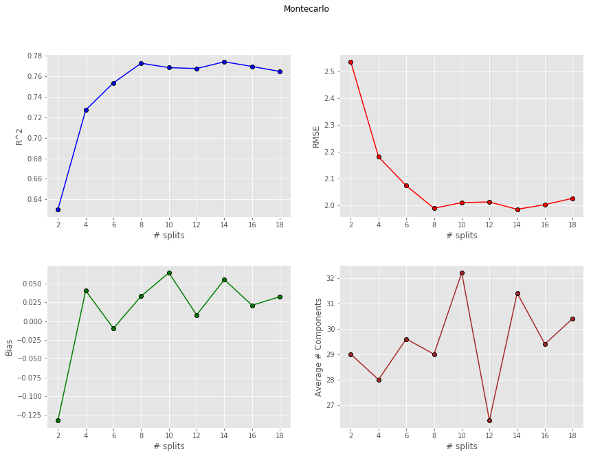
Then Montecarlo
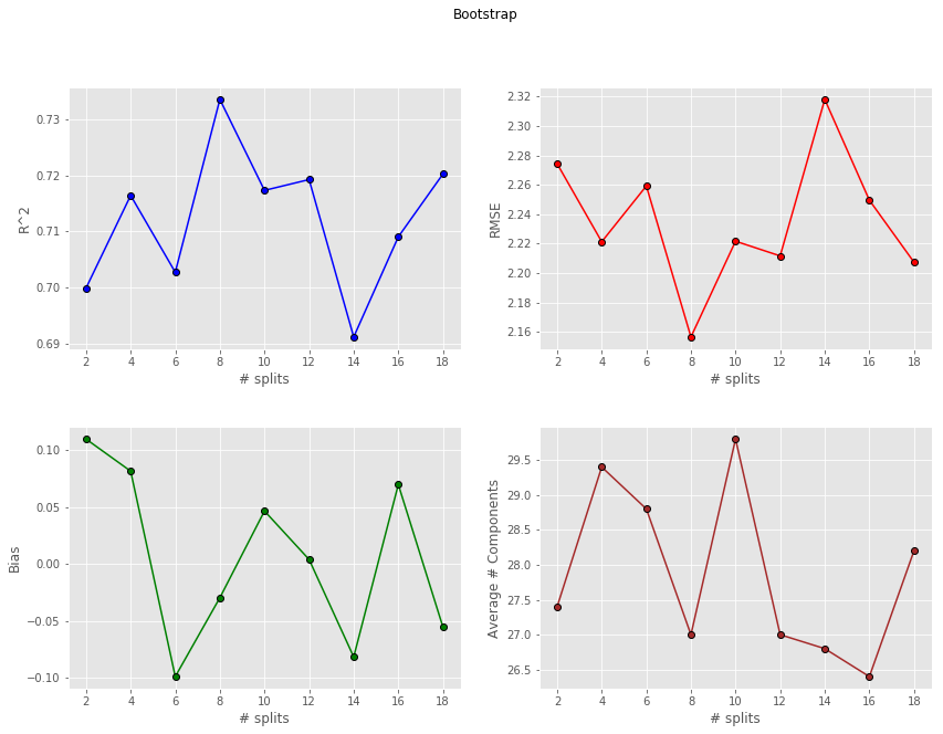
and finally Bootstrap
Comparison and wrap-up
K-Fold and Montecarlo give quite comparable performances. If anything Montecarlo tends to be a bit more repeatable (less variance) due to the fact that we have enough samples to generate statistically different splits. The bias however is generally higher than the corresponding value for K-Fold. This thing is well known in machine learning. In fact it’s got a name: it’s called Bias-Variance tradeoff.
Bootstrap doesn’t seem to perform as good. In fact Bootstraps metrics don’t really change with increasing the number of splits, and they’re worse than the corresponding values for K-Fold and Montecarlo. The likely reason for this is the repetition of spectra in any one Bootstrap training set. More precisely, the number of samples in this case is not large enough to guarantee a satisfactory model using the training set alone. Therefore all Bootstrap models tend to be inferior in robustness compared to the other CV methods.
Anyway, we have covered a few ways to build a cross-validation procedure for your spectroscopy data. Truth be told, K-Fold CV is going to be pretty good in most cases, but by using the ideas in this post, you can build more versatile approaches for your cross-validation implementations.
Hope you enjoyed the post. If you found it useful, please share it with a friend or colleagues and help us grow. Bye for now and thanks for reading!