Baseline correction refers to a set of preprocessing techniques for spectroscopy. The basic idea is that a spectrum contains features of interest and a background.
The features (peaks, for instance) are related to the sample properties we want to analyse, while the background can be caused by factors like detector noise, scattering, etc which are not related to the properties we want to study.
The aim of baseline correction techniques is to remove this background signal to isolate just the peaks.
In this post we are going to look at two approaches for baseline correction. The first is based on wavelet transform (WT), and the second on asymmetric least squares (ALS).
We will apply the two methods to two different datasets: a Raman spectrum and an X-ray Fluorescence (XRF) spectrum.
The method based on WT has the advantage to be easily explainable in terms of the underlying properties of the wavelet decomposition. We will see however, that the results are not that good. The ALS method may be less intuitive, but produces a much better result.
Method 1: baseline correction using wavelet transform
We discussed wavelets transforms on Nirpy Research in the context of spectra denoising. Wavelet decompositions have the appealing properties of being able to select different components of a given spectrum, from the sharp features down to the more gentle variations.
Wavelet-based denoising of a NIR spectrum is the process of identifying the very sharp characteristic in it and removing them. Remember that generally NIR spectra have broader features, not very sharp ones, therefore it’s likely that sharp features are generated by random noise, and removing them leads to de-noising.
The process of baseline correction is in many respects, the opposite of denoising. Here we want to identify (and remove) a broad baseline and keep the sharp features. So the process of baseline correction with a wavelet decomposition follows exactly the steps of the denoising posts, except that it is the low-frequency features that are removed.
This is the idea behind the paper Automatic Baseline Correction by Wavelet Transform for Quantitative Open-Path Fourier Transform Infrared Spectroscopy by Shao and Griffiths.
Method 2: baseline correction by asymmetric least squares
The idea is to derive a smooth functions that follows the baseline of a spectrum. To achieve that, one could start from a smooth function that fits the entire spectrum (including the peaks), and then calculating the deviations (either positive or negative) from the fitted function.
Peaks will have a positive deviations while the baseline points will have negative deviations. The key idea behind ALS is that it applies different penalties to positive and negative deviations when fitting. Specifically, one penalises the positive deviations much more than the negative deviations.
In this way, the fit will ‘neglect’ the peaks and adapt much better to the baseline points, which are much less penalised.
What we described here is an iterative procedure, which starts from a flat baseline, applies penalties as described and repeat the fit for a specified number of iterations.
Interlude: X-ray Fluorescence (XRF)
Before getting stuck into the details of baseline correction methods, let’s spend a few words on XRF.
X-Ray Fluorescence (XRF) is a form of spectroscopy that uses high-energy x-ray photons to probe the elemental composition of a sample.
The main advantage of XRF compared to vibrational spectroscopy techniques (such as NIR spectroscopy) is that x-rays interacts with inner shell electrons in material. These electrons are (typically) never shared in chemical bonds, hence their characteristic transitions are a signature of the elemental composition of a sample, nearly independent from its chemical state.
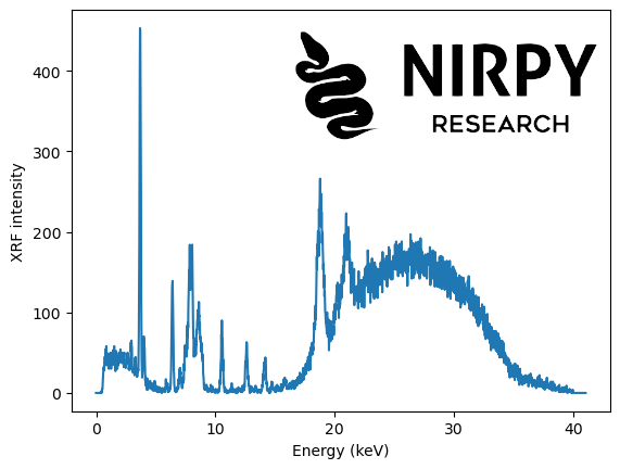
XRF data is characterised by sharp peaks (corresponding to characteristic energy transitions of inner shell electrons) overlapping a slowly varying (broadband) baseline generated by the so called bremsstrahlung (braking radiation).
Imports and Data
Here’s the list of the imports
|
1 2 3 4 5 6 7 8 9 10 11 |
import pandas as pd import numpy as np import matplotlib.pyplot as plt # Needed for wavelet decomposition import pywt # Nedded for ALS from scipy import sparse from scipy.linalg import cholesky from scipy.sparse.linalg import spsolve |
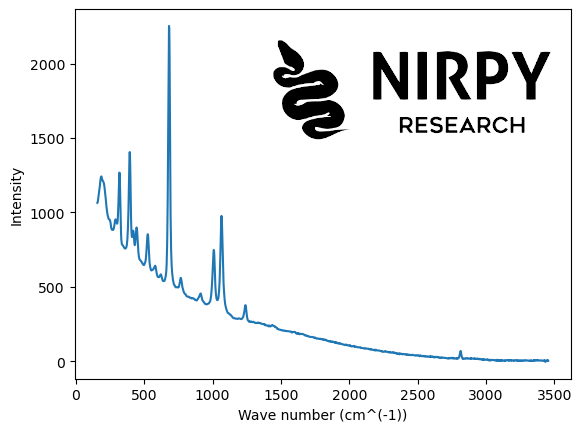
The Raman spectrum is from a sample of Beryl as available on the RRUFF repository. A direct link to the dataset in text format is at this link.
Here’s the code to read out the Raman data and the associated wavenumbers from the file.
|
1 2 3 4 5 6 7 8 9 10 11 12 13 14 15 16 17 18 19 20 21 22 23 24 25 26 |
fn = "Beryl__R110118__Broad_Scan__780__0__unoriented__Raman_Data_RAW__22217.rruff" lines = [] with open(fn) as f: lines.append(f.readlines()) wavenumb = [] raman = [] for i,j in enumerate(lines): wn = [] rm = [] for l, line in enumerate(j[10:]): if line == '##END=\n': break else: wn.append(float(line.split(',')[0])) rm.append(float(line.split(',')[1])) wavenumb.append(wn) raman.append(rm) wn = np.array(wavenumb[0]) raman = np.array(raman[0]) plt.plot(wn, raman) plt.xlabel("Wave number (cm^(-1))") plt.ylabel("Intensity") plt.show() |
The XRF data is from a sample of ink and it was downloaded from this Mendeley repository, related to the paper “XRF elemental analysis of inks in South American manuscripts from 1779 to 1825” by C. L. Obregon et al.
|
1 2 3 4 5 6 7 8 9 10 |
data = pd.read_excel('Raw data-ancient inks_16Ene2021.xlsx', sheet_name = 'spectra data', \ usecols="A:C", skiprows=1, header=None ) xrf = data[2][20:].values energy = data[2][2] + data[2][3]*np.arange(xrf.shape[0]) plt.plot(energy, xrf) plt.xlabel("Energy (keV)") plt.ylabel("XRF intensity") plt.show() |
Baseline correction by wavelet decomposition
Our approach to baseline correction by wavelet decomposition closely mirrors the algorithm for denoising described in a previous post. The first step is identical: the spectra are decomposed with a wavelet type of choice. The second step is different. Since we aim at removing a baseline (slowly varying contribution) we would like to suppress the lowest order of the wavelet decomposition (in denoising we suppress the highest order instead).
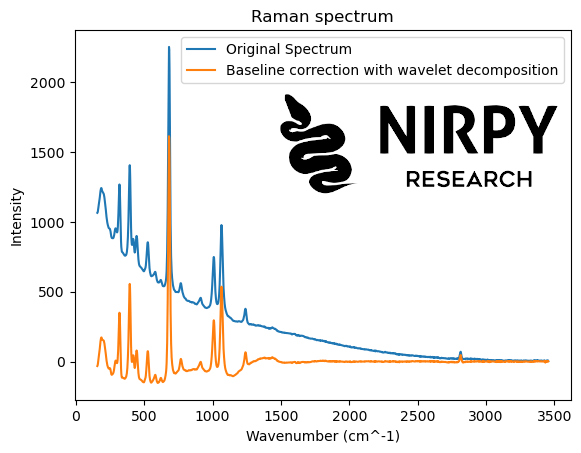
Here’s how the algorithm looks for the Raman spectrum
|
1 2 3 4 5 6 7 8 9 10 11 12 13 14 15 16 17 18 |
wavelet_type = 'db6' # Wavelet transform coeffs_raman = pywt.wavedec(raman, wavelet_type, level = 7) # Inverse wavelet transform new_coeffs_raman = coeffs_raman.copy() new_coeffs_raman[0] = 0*new_coeffs_raman[0] # Inverse wavelet transform new_raman = pywt.waverec(new_coeffs_raman, wavelet_type) plt.plot(wn, raman, label = 'Original Spectrum') plt.plot(wn, new_raman, label = 'Baseline correction with wavelet decomposition') plt.xlabel("Wavenumber (cm^-1)") plt.ylabel("Intensity") plt.title("Raman spectrum") plt.legend() plt.show() |
and similarly for the XRF spectrum
|
1 2 3 4 5 6 7 8 9 10 11 12 13 14 15 16 17 18 |
wavelet_type = 'db6' # Wavelet transform coeffs_xrf = pywt.wavedec(xrf, wavelet_type, level = 7) # Set to zero the first coefficient new_coeffs_xrf = coeffs_xrf.copy() new_coeffs_xrf[0] = 0*new_coeffs_xrf[0] # Inverse wavelet transform new_xrf = pywt.waverec(new_coeffs_xrf, wavelet_type) plt.plot(energy, xrf, label = 'Original Spectrum') plt.plot(energy, new_xrf, label = 'Baseline correction with wavelet decomposition') plt.xlabel("Energy (keV)") plt.ylabel("XRF intensity") plt.title("XRF spectrum") plt.legend() plt.show() |
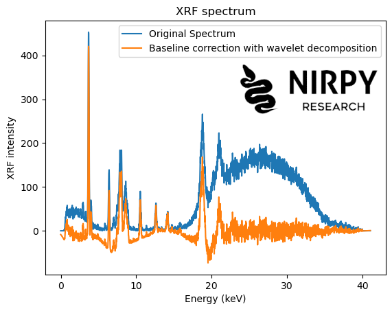
In both cases, the simple procedure of setting to zero the first wavelet coefficient is fairly effective at getting rid of most of the baseline. Some distortions however are present: in some cases the new baseline is not completely flat, it dips below zero or the correction overshoots in the vicinity of some of the peaks.
In fairness, the procedure of setting to zero the first WT coefficient (and leaving the others unchanged) is fairly crude. Improvements can be made, for instance by smoothly decreasing the amplitude of the lower-order coefficients, or playing around with the wavelet type. But (as they say in the good books) I leave this for the interested reader to explore.
Baseline correction with asymmetric least squares
There are many versions (and variations) of ALS for baseline correction. We are going to refer to the functions provided in the irfpy.ica library published by the Swedish Institute of Space Physics (copyright Yoshifumi Futaana, Martin Wieser, and Gabriella Stenberg Wieser), and specifically to the code available at this page.
We are going to use the als and arpls functions, which are reproduced at the end of this post. The als function is the original version of the ALS algorithm (as briefly described above). The ARPLS algorithm is similar, but the asymmetric weights are iteratively adjusted.
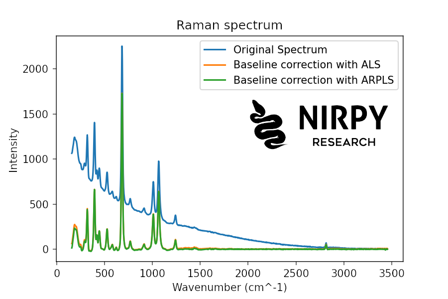
Here’s the code to correct the Raman spectrum (note that the functions calculate the baseline, which can be then subtracted from the original spectrum)
|
1 2 3 4 5 6 7 8 9 10 11 |
baseline_als_raman = als(raman, lam=1e6, niter=5) baseline_arpls_raman = arpls(raman, lam=1e6, niter=5) plt.plot(wn, raman, label = 'Original Spectrum') plt.plot(wn, raman - baseline_als_raman, label = 'Baseline correction with ALS') plt.plot(wn, raman - baseline_arpls_raman, label = 'Baseline correction with ARPLS') plt.xlabel("Wavenumber (cm^-1)") plt.ylabel("Intensity") plt.title("Raman spectrum") plt.legend() plt.show() |
 And here’s the corresponding code for XRF
|
1 2 3 4 5 6 7 8 9 10 11 |
baseline_als_xrf = als(xrf, lam=1e6, niter=5) baseline_arpls_xrf = arpls(xrf, lam=1e6, niter=5) plt.plot(energy, xrf, label = 'Original Spectrum') plt.plot(energy, xrf - baseline_als_xrf, label = 'Baseline correction with ALS') plt.plot(energy, xrf - baseline_arpls_xrf, label = 'Baseline correction with ARPLS') plt.xlabel("Energy (keV)") plt.ylabel("XRF intensity") plt.title("XRF spectrum") plt.legend() plt.show() |
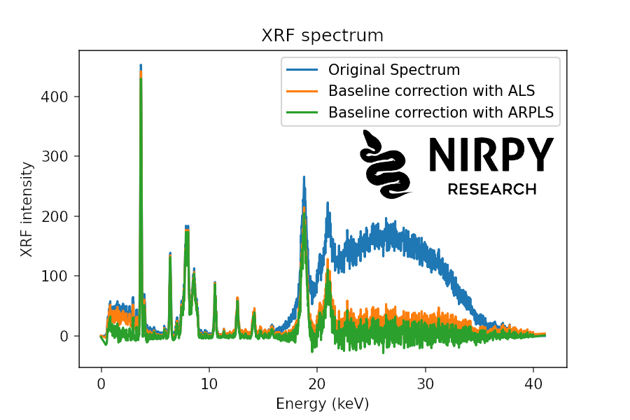
In both cases the result is much neater even for the XRF spectrum showing a much larger noise compared to the Raman spectrum.
As always, thanks for reading until the end and until next time.
Daniel
References and links
- Cover image adapted from an original photo by Eberhard Grossgasteiger on Pexels
- XRF data from Zamalloa Jara et al. (2023), “Elemental analysis XRF of inks (1778-1825) ”, on Mendeley Data
- XRF data discussed in the paper by Luízar Obregón et al. (2021). XRF elemental analysis of inks in South American manuscripts from 1779 to 1825, on Herit Sci
- ALS and ARPLS code by M. Wieser available here.
- Beryl Raman spectrum data from the RRUFF database available here.
Appendix: Original ALS and ARPLS by M. Wieser
Redistributed under the terms of the GNU Lesser General Public License.
|
1 2 3 4 5 6 7 8 9 10 11 12 13 14 15 16 17 18 19 20 21 22 23 24 25 26 27 28 29 30 31 32 33 34 35 36 37 38 39 40 41 42 43 44 45 46 47 48 49 50 51 |
def als(y, lam=1e6, p=0.1, itermax=10): r""" Implements an Asymmetric Least Squares Smoothing baseline correction algorithm (P. Eilers, H. Boelens 2005) Baseline Correction with Asymmetric Least Squares Smoothing based on https://web.archive.org/web/20200914144852/https://github.com/vicngtor/BaySpecPlots Baseline Correction with Asymmetric Least Squares Smoothing Paul H. C. Eilers and Hans F.M. Boelens October 21, 2005 Description from the original documentation: Most baseline problems in instrumental methods are characterized by a smooth baseline and a superimposed signal that carries the analytical information: a series of peaks that are either all positive or all negative. We combine a smoother with asymmetric weighting of deviations from the (smooth) trend get an effective baseline estimator. It is easy to use, fast and keeps the analytical peak signal intact. No prior information about peak shapes or baseline (polynomial) is needed by the method. The performance is illustrated by simulation and applications to real data. Inputs: y: input data (i.e. chromatogram of spectrum) lam: parameter that can be adjusted by user. The larger lambda is, the smoother the resulting background, z p: wheighting deviations. 0.5 = symmetric, <0.5: negative deviations are stronger suppressed itermax: number of iterations to perform Output: the fitted background vector """ L = len(y) D = sparse.eye(L, format='csc') D = D[1:] - D[:-1] # numpy.diff( ,2) does not work with sparse matrix. This is a workaround. D = D[1:] - D[:-1] D = D.T w = np.ones(L) for i in range(itermax): W = sparse.diags(w, 0, shape=(L, L)) Z = W + lam * D.dot(D.T) z = spsolve(Z, w * y) w = p * (y > z) + (1 - p) * (y < z) return z |
|
1 2 3 4 5 6 7 8 9 10 11 12 13 14 15 16 17 18 19 20 21 22 23 24 25 26 27 28 29 30 31 32 33 34 35 36 37 38 39 40 41 42 43 44 45 46 47 48 49 50 51 52 53 54 55 56 57 58 |
def arpls(y, lam=1e4, ratio=0.05, itermax=100): r""" Baseline correction using asymmetrically reweighted penalized least squares smoothing Sung-June Baek, Aaron Park, Young-Jin Ahna and Jaebum Choo, Analyst, 2015, 140, 250 (2015) Abstract Baseline correction methods based on penalized least squares are successfully applied to various spectral analyses. The methods change the weights iteratively by estimating a baseline. If a signal is below a previously fitted baseline, large weight is given. On the other hand, no weight or small weight is given when a signal is above a fitted baseline as it could be assumed to be a part of the peak. As noise is distributed above the baseline as well as below the baseline, however, it is desirable to give the same or similar weights in either case. For the purpose, we propose a new weighting scheme based on the generalized logistic function. The proposed method estimates the noise level iteratively and adjusts the weights correspondingly. According to the experimental results with simulated spectra and measured Raman spectra, the proposed method outperforms the existing methods for baseline correction and peak height estimation. Inputs: y: input data (i.e. chromatogram of spectrum) lam: parameter that can be adjusted by user. The larger lambda is, the smoother the resulting background, z ratio: wheighting deviations: 0 < ratio < 1, smaller values allow less negative values itermax: number of iterations to perform Output: the fitted background vector """ N = len(y) D = sparse.eye(N, format='csc') D = D[1:] - D[:-1] # numpy.diff( ,2) does not work with sparse matrix. This is a workaround. D = D[1:] - D[:-1] H = lam * D.T * D w = np.ones(N) for i in range(itermax): W = sparse.diags(w, 0, shape=(N, N)) WH = sparse.csc_matrix(W + H) C = sparse.csc_matrix(cholesky(WH.todense())) z = spsolve(C, spsolve(C.T, w * y)) d = y - z dn = d[d < 0] m = np.mean(dn) s = np.std(dn) wt = 1. / (1 + np.exp(2 * (d - (2 * s - m)) / s)) if np.linalg.norm(w - wt) / np.linalg.norm(w) < ratio: break w = wt return z |