Classification of NIR spectra by Linear Discriminant Analysis in Python

Products or raw materials identification is one of the staples of NIR analysis in industrial processing. Identification of a product or substance – or detection of anomalies over the expected range – are usually accomplished by separating NIR spectra into different classes. In this post we’ll work through an example of classification of NIR spectra by Linear Discriminant Analysis in Python.

What is Linear Discriminant Analysis?

Linear Discriminant Analysis (or LDA from now on), is a supervised machine learning algorithm used for classification. True to the spirit of this blog, we are not going to delve into most of the mathematical intricacies of LDA, but rather give some heuristics on when to use this technique and how to do it using scikit-learn in Python.

Before we start, I’d like to mention that a few excellent tutorials on LDA are already available out there. Most notably, check out a 2014 blog post by Sebastian Raschka available here, that was an inspiration for this post.

When it comes to explaining LDA, the usual approach is to compare it with the good old Principal Component Analysis (PCA) to remark similarities and differences. Well, this is exactly what we are going to do here, but we’ll show how LDA is not necessarily an alternative to PCA, but they can actually work together.

But I’m getting ahead of myself. Let’s recap what we covered about PCA (for a refresher, take a look at these posts).

• Intro to PCA
• PCA classification of NIR spectra
• NIR classification of macadamias

PCA is a dimensionality reduction technique. Restricting our attention to NIR analysis, PCA will get rid of correlated components in the data (for instance absorbance at different wavelength bands) by projecting such multidimensional data to a much lower dimensionality space. The projected components (ahem, principal components) are now independent and are chosen in order to maximise the variance of the data.

As such, PCA is an unsupervised machine learning method, that is it takes into account only the spectral data (and its variance) and not the labels that may be available.

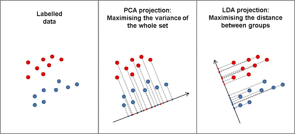
Conversely, LDA makes use of the labels to produce a dimensionality reduction that is designed to maximise the distance between the classes. Let’s repeat this once again: PCA will find the projections that maximise the variance of the data regardless of their grouping. LDA will try and maximise the distance between those groups.

Now, all these concepts have a precise mathematical definition but, as the old adage goes, let’s try to save a thousand more words and look at the picture below. Just so you know it, this picture is totally made up with the only purpose of clarifying the difference between PCA and LDA.

One may naively think then, that when labels are available, LDA is necessarily superior to PCA, because for once it uses all of the available information. That is not necessarily true however, and we’ll see here how this is very pertinent for NIR analysis.

OK, after this important introduction, let’s go ahead and work with LDA in Python.

Linear Discriminant Analysis in Python

With my consulting business (Instruments & Data Tools), I once worked on a lab test to detect allergens using NIR analysis. For that exercise, we mixed milk powder and coconut milk powder with different ratios, from 100% milk powder to 100% coconut milk powder in increments of 10%. We then acquired absorbance spectra and verified how the NIR spectra correlate to the different composition of the samples. The data is available for download at our Github repository.

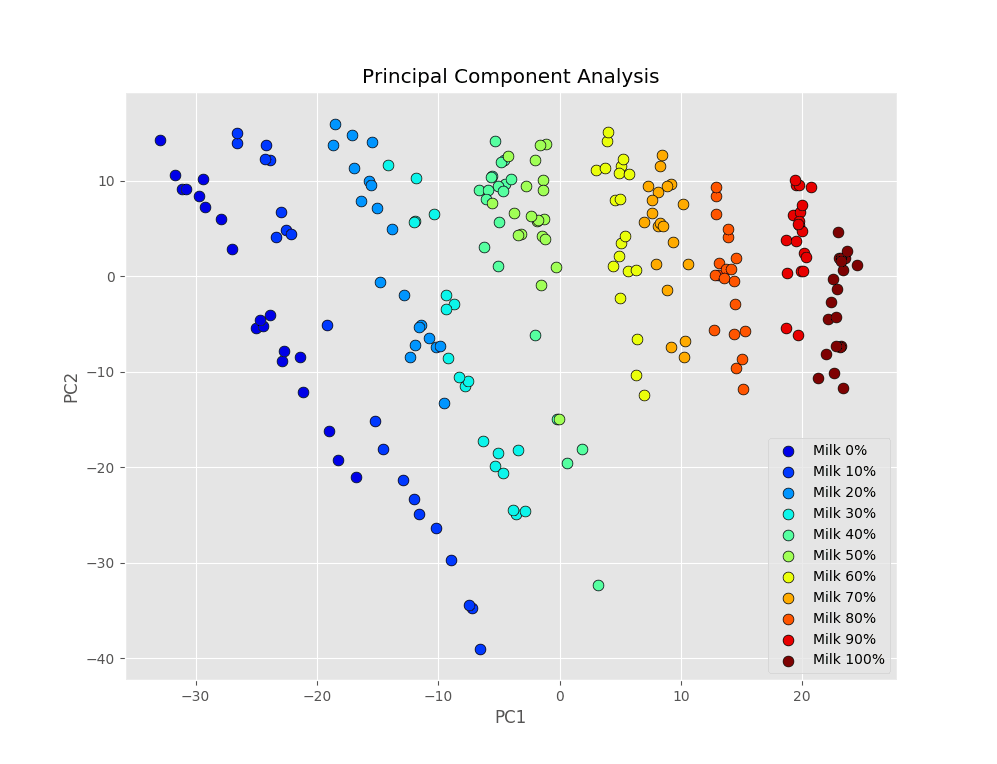
In this case PCA gives us a neat classification of the spectra. Here’s the scatter plot of the first two principal components, as we showed in that post.
The different groups of measurements are mostly separated from one another, with a few overlaps. For instance data from 20% milk and 30% milk powder overlap quite a bit, and the same happens for 40% and 50% milk. This situation is what we are referring to when we say that PCA finds the directions where the variance of the data is maximised. Even though spectra are naturally segregated, because of the nature of the samples we measured,  tha32qqqat may not be evident along the directions of maximal variance.

LDA can produce data segregation in a much more efficient manner, since it makes use of the labels we have about the data. Implementing LDA is a matter of a couple of lines in Python.

And here’s the result.Pretty stunning difference, isn’t it? Spectra corresponding to the same milk/coconut milk powder ratio cluster neatly when transformed with LDA. However, let’s stress that there is nothing magical about this. LDA uses the labels associated with the scans, so the algorithm knows exactly which scan belongs to which group.

There is one thing however that you’ll notice as soon as you run the code above: a warning is generated. The warning looks something like this:

Don’t worry about it just yet. We’ll come back to that before the end of the post.

For the moment, let’s use the classification accuracy of LDA to build a genuine classifier.

NIR spectra classifier using LDA in Python

The previous code snippet is applying LDA on the whole dataset. Since we knew the labels already, that is not of much use really. The true advantage of having this tool is to be able to make predictions on unknown samples.

To simulate this process we divide our data into a training set and a test set. The LDA is trained only on the training set (I know, I know, just in case…) and the test set is used to verify the accuracy of the classification.

In Python that looks something like this.

Let’s go over this code bit by bit. The key imports here are train_test_split (with obvious meaning) and cross_val_score (which we’ll use later).

In the second line we split the dataset into train and test set, reserving 25% of our data (test_size) to the test set. The split is normally done randomly. If you want it to be repeatable (for instance if you want to check the performance of the classifier on the same split by changing some other parameter), just specify the random_state value to some number. Otherwise omit that entirely.

Now we are ready to train our classifier. This is done with the lda.fit command. Note that, unlike what we have done before, we are not using the lda.fit_transform command. In fact, we are not looking at generating a new dataset with reduced dimensionality, but at training our LDA classifier.

OK, once the classifier is trained we can test the performance of the model by predicting the results on the test set, and checking the accuracy of the prediction with the (known) labels of the test set with the command lda.score.

The result I get in my case is not bad at all. That’s the output of the script

Very good, we reached 98% classification accuracy on the test set, which is a pretty good result.

However, you may argue that this good result may just be an accident of the specific split we have done. In other words, we may have just been lucky. To rule out this possibility we use the  cross_val_score function we introduced before. The code goes like this

In this case we don’t have to specify a test-train split. This is done automatically by specifying the number of “folds”, that is the number of splits in our data. For instance, by specifying cv=4 we are dividing our data in 4 parts, train the classifier on three of them and use the last part for test. The entire procedure is then repeated by choosing a different test set.

In this way we can get an average of more than one run, which is guaranteed to give a better estimation of the accuracy of our classifier. In my case that’s what I get.

It is still pretty good, but clearly we have to admit that the single split we have done before was something of a lucky run.

Anyway, this would be it, if it wouldn’t be for that nagging warning we keep getting. Variables are collinear! It’s time to fix that.

If you’ve been paying attention, we mentioned a few times that NIR spectra suffer from collinearity problems. Collinearity means that the value of the spectra (the “samples” in machine learning lingo) at different wavelengths (the “features”) are not independent, but highly correlated. This is the reason for the warning.

Again, if you’ve been paying attention, you’d also remember that PCA is one of the ways to remove collinearity problems. The individual principal components are always independent from one another, and by choosing a handful of principal components in our decomposition we are guaranteed that collinearity problem is eliminated.

So it’s time to bring back good old PCA and see how we can combine PCA with LDA.

Combining PCA and Linear Discriminant Analysis

In many places across the internet we are left with the impression that PCA and LDA are kind of alternatives. We have discussed however that they are really two different beasts, and in fact we can combine  them to make our classification even better.

The idea is simple. Let’s extract a handful of principal components from our data, and use those as input for our classifier. In this case we solve the collinearity problem, and we achieve a better accuracy as well!

Here’s the code

And here’s the result

Very pleasing. We got our 98% accuracy back, this time as an average of a few splits. And, most importantly, no warning is generated this time!

As an aside, I have just decided to use 15 principal components, but this value is by no mean optimised. I would expect that there is an optimal value for the number of components. Using too few components will not capture the whole variance in the data. Using too many of them would give as a result that tends to the one using the whole spectra. Anyway, I leave the optimisation exercise to you.

For now, thanks for tuning in and I hope that as been useful. As usual feel free to give us a shout if you have any doubt, or spotted any problems with this code. Until next time!