In 2003, Paul Eilers published a paper titled “A Perfect Smoother” [1], re-implementing and extending early ideas published by Whittaker in the 1920s [2].
The method is based on a penalised least square approach, also called Tikhonov regularization (also called ridge regression!) and is a very general approach to deal with smoothing noisy data, overcoming some of the limitations of the Savitzky-Golay method. The specific smoothing method first introduced by Whittaker is also referred to as Whittaker-Henderson smoothing or Whittaker-Eilers smoothing or Hodrick-Prescott filter.
In this post, I’m digging into the mathematical formulation of Whittaker smoothing, and putting it in a form that is easy to implement for spectroscopy. This post has a mathematical introduction, which I tried to keep as simple as possible, and its implementation in Python. The approach presented here has many interesting ramifications; at the end of the post, I wrote a few open questions which I plan to revisit in the future.

Tikhonov regularization (aka ridge regression)
Tikhonov regularization is a general method for solving ill-posed problems. A classic example of this ill-posedness is solving a least-square problem with near-infrared (NIR) spectra. If X is the matrix of observations (spectra) and y is the target variable, an ordinary least-square problem is to find a set of coefficients w such that y = Xw.
The optimal least-square solution is the one that minimises the squared norm ||y- Xw||^{2}.
In mathematical notation the solution is
\hat{w} = \mathrm{arg min}_{w} ||y- Xw||^{2}, where the ‘hat’ symbol on top of \hat{w} is there to indicate that the solution is a ‘best fit’ to w, which minimises the squared norm, but generally not identical to w.
Working through the maths (which you can find on the Wikipedia page on linear regression), the solution to this problem is:
\hat{w} = \left( X^{T} X \right)^{-1} X^{T} y,
where X^{T} is the transpose of X and the exponent -1 means the inverse matrix.
When X is a matrix of NIR spectra the problem is ill-posed because adjacent wavelengths often contain very similar information, leading to high correlation between predictors. The consequence is that the matrix X^{T} X is almost singular, hence its inverse does not exist.
In such conditions, the least-squares problem becomes numerically highly unstable.
The typical workaround is to use a suitable decomposition of X, such as PCA or PLS and then solve a least-squares problem on the coefficients.
Another possible approach is a penalised (aka regularised) least-squares, whereby a penalty term is added to the quantity to be minimised, such that it imposes the further constraint that the squared norm of the coefficients is small. This is what is normally called Tikhonov regularisation, or ridge regression.
Mathematically, a penalty term \lambda ||w||^2 is added to the quantity to be minimised, with \lambda being a tunable parameter. The solution to the regularised problem becomes
\hat{w} = \mathrm{arg min}_{w} \left( ||y- Xw||^{2} + \lambda ||w||^2 \right).
The penalty term prevents the quantity ||w||^2 (or, more precisely, ||\hat{w}||^2 ) from becoming too large, thus stabilising the numerical approach.
Whittaker smoothing
The smoothing technique proposed by Whittaker is very similar to what we just described, but with some important differences (and some changes in notation). Let’s follow the (extremely clear) explanation by Eilers.
Assume that x is a measured NIR spectrum (we use the lower-case notation, as opposed to X, to indicate that we are dealing with a single spectrum) and x_{s} is a smoothed version of it, which we want to calculate. What are the requirements on x_{s}?
- First, we want x_{s} to be “not too different” from x. We can impose this constraint by requiring the squared norm ||x - x_{s}||^2 to be small. To make this look like the least-squares problem of the previous section, we can insert an identity matrix I so that the squared norm is equivalently written as ||x - I x_{s}||^2.
- Second, we want x_{s} to be smooth (of course). This constraint can be imposed by minimising the second derivative of x_{s}, which can be thought of as a measure of its ‘roughness’. If we write the second derivative as an operator D_{2} acting on x_{s}, we require the squared norm ||D_{2}x_{s}||^2 to be small.
Putting these things together, we have
\hat{x}_{s} = \mathrm{arg min}_{x_{s}} \left( ||x - I x_{s}||^{2} + \lambda ||D_{2}x_{s}||^2 \right).
The solution \hat{x}_{s} to this problem is the smooth spectrum we are after.
Following the derivation by Eilers, the solution is
\hat{x}_{s} = S_{\lambda} x,
where we have defined the smoothing kernel S_{\lambda} = \left(I + \lambda D_{2}^{T} D_{2}\right)^{-1} . As we are about to see, this problem can be easily solved using the relevant linear algebra routines implemented in Numpy.
Python implementation of the Whittaker smoother
Let’s start with importing the required libraries and loading a dataset:
|
1 2 3 4 5 6 7 8 9 10 11 12 13 14 15 16 17 |
import numpy as np import pandas as pd import matplotlib.pyplot as plt import re,glob def natural_sort(l): convert = lambda text: int(text) if text.isdigit() else text.lower() alphanum_key = lambda key: [convert(c) for c in re.split('([0-9]+)', key)] return sorted(l, key=alphanum_key) # Import the data fl = natural_sort(glob.glob("./Avocado_NIR_scans/Avocado_spectra/*csv")) spectra = np.zeros((len(fl), 228)) for i,j in enumerate(fl): spectra[i,:] = pd.read_csv(j, skiprows=21)['Absorbance (AU)'] wavelength = pd.read_csv(j, skiprows=21)['Wavelength (nm)'] |
The dataset is available as a zip file in our GitHub repository. It contains 100 NIR spectra of a Hass avocado. For the purpose of illustrating Whittaker smoothing, we’ll just use one of the spectra for now. Here’s the complete Whittaker algorithm, with all the quantities defined in the comments.
|
1 2 3 4 5 6 7 8 9 10 11 12 |
# number of wavelengths n = spectra.shape[1] # Second derivative operator D2 = np.diff(np.eye(n), 2, axis=0) # Regularization parameter -- this can be tuned lambda_reg = 1 # Identity matrix I = np.eye(n) # Smoothing kernel S_lambda = np.linalg.inv(I + lambda_reg * (D2.T @ D2)) # Smoothed spectrum x_s = S_lambda @ spectra[0,:] |
Here’s a plot of the smoothed spectrum overlapping the original spectrum:
|
1 2 3 4 5 6 7 |
plt.figure(figsize=(7, 4)) plt.plot(wavelength, spectra[0,:], label='Sample Spectrum') plt.plot(wavelength, x_s, label='Whittaker-smoothed spectrum with $ \\lambda = 1$') plt.xlabel('Wavelength (nm)') plt.ylabel('Absorbance') plt.legend() plt.show() |
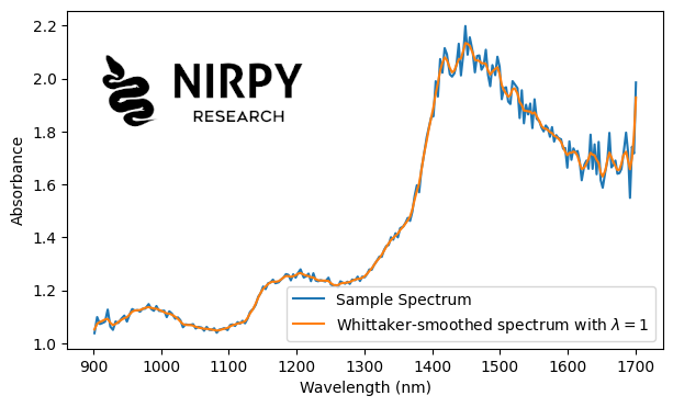
The implementation of the Whittaker smoothing algorithm is really quite simple. However, a good smoothing filter depends on the correct choice of the regularisation parameter \lambda. The value \lambda = 1 chosen above is a reasonable estimate, but it was chosen only according to a visual inspection of the smoothed spectrum.
There are a few ways to select the optimal \lambda. Here, I’m going to present a heuristic method called the “L-curve” which has general applicability in penalised regression problems. In the next section, I will discuss the method and its limitations.
Choosing the regularisation parameter with the L-curve method
The L-curve is a graphical tool to estimate the optimal value of the penalty term \lambda in a regularised regression problem. Its name is derived from the typical shape of the curve, reminiscent of the capital letter “L”.
The curve is a parametric log-log plot of the term \eta = ||D_2 x_{s}|| versus \rho = || x - x_{s} || (alternatively, it can be a linear-scale plot of \log \eta versus \log \rho ) by varying \lambda. Here’s an implementation:
|
1 2 3 4 5 6 7 8 9 10 11 12 13 14 15 |
# Define the set of lambdas in log scale lambdas = np.logspace(-1,5,1000) rho = np.zeros(len(lambdas)) eta = np.zeros(len(lambdas)) for i, lam in enumerate(lambdas): S_lambda = np.linalg.inv(I + lam * (D2.T @ D2)) x_s = S_lambda @ spectra[0,:] rho[i] = np.linalg.norm(spectra[0,:] - x_s) eta[i] = np.linalg.norm(D2 @ x_s) plt.loglog(rho, eta) plt.xlabel("$ \\rho = ||x - x_{s} ||$") plt.ylabel("$ \\eta = ||D_2 x_{s}||$") plt.show() |
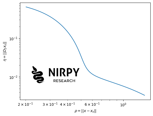
Let’s study the shape of the curve for the purpose of finding the optimal value for the regularisation parameter. When \lambda is very small, we are in the top-left of the plot. In these conditions there is no smoothing, hence x_{s} \approx x and \rho \approx 0 . At the opposite end, when \lambda is very large, the spectrum is over-smoothed, hence its roughness \eta \approx 0 but \rho is large.
Intuitively, in the region between these two extremes, one can find a point where these two effects are balanced. This is the “knee” of the L-curve, which in our plot above sits where \rho \approx 5.5 .
As you no doubt have observed, the shape of our curve above is not really like a “L”. This contrasts with other examples you can find online, for instance the (excellent) lecture by Prof. Per Christian Hansen available here (other criteria for choosing \lambda are also described in this lecture). The L-curve you see plotted in slide 14 of this lecture, has a very sharp corner, significantly different from the one calculated in our case. The discrepancy will depend on the structure of the noise, and the underlying signal, we are dealing with. The more gently-varying is the (noiseless) signal, the less pronounced will be the knee of the L-curve. Hence the applicability of this heuristic method should be evaluated on each case.
Let’s keep this in mind and move on with the description of the method. The knee of the L-curve will be the point of maximum curvature within a suitable range of values of \lambda. Again referring to the lecture notes linked above, the curvature is defined by
\hat{c}_{\lambda} = 2 \frac{\hat{\rho}' \hat{\eta}'' - \hat{\eta}' \hat{\rho}''}{\left[ (\hat{\rho}')^{2} + \hat{\eta}')^{2} \right]^{3/2}}.
In the previous formula, \hat{\rho} = \log \rho, \hat{\eta} = \log \eta, the primes denote differentiation with respect to \lambda and the double prime means second derivative. We can therefore implement this formula and looks for the maximum.
|
1 2 3 4 5 6 7 8 9 10 11 12 13 14 15 16 17 18 19 20 21 22 23 24 25 |
def L_curve_knee(lambdas, rho, eta): """ Find the corner of the L-curve (max curvature) in log-log space. See details here: https://people.compute.dtu.dk/pcha/DIP/chap5.pdf """ rho_hat = np.log(rho) eta_hat = np.log(eta) # First derivatives. Use log lambdas since lambdas are defined as np.logspace d_rho_hat = np.gradient(rho_hat, np.log(lambdas)) d_eta_hat = np.gradient(eta_hat, np.log(lambdas)) # Second derivatives dd_rho_hat = np.gradient(d_rho_hat, np.log(lambdas)) dd_eta_hat = np.gradient(d_eta_hat, np.log(lambdas)) # Curvature formula from the link above numerator = d_rho_hat * dd_eta_hat - dd_rho_hat * d_eta_hat denominator = (d_rho_hat**2 + d_eta_hat**2) ** 1.5 curvature = 2* numerator / denominator knee_loc = np.argmax(np.abs(curvature)) optimal_lambda = lambdas[knee_loc] return curvature, optimal_lambda, knee_loc |
Note that the function above assumes that the array lambdas is defined in logarithmic space, as we did above. If the spacing between the elements of lambdas is logarithmic, then the spacing between the elements of np.log(lambdas) is approximately linear, which makes it suitable to be used as argument for the np.gradient() function. If the array lambdas is defined in linear space, the function above must be modified accordingly.
One more thing to note is that the derivative with respect to \log \lambda (as used in the function above) is obviously different from the derivative with respect to \lambda, which is assumed in the formula for \hat{c}_{\lambda} . However, using the chain rule and substituting the results in the curvature formula above, you’ll work out that the expression for the curvature is unchanged, if the derivatives are done with respect to \log \lambda, as the extra factors cancel out.
With these explanations in mind, here’s the script.
|
1 2 3 4 5 6 7 8 9 10 11 12 13 14 15 16 17 18 19 |
curvature, optimal_lambda, knee_loc = L_curve_knee(lambdas, rho, eta) # Smoothing kernels S_opt_lambda = np.linalg.inv(I + optimal_lambda * (D2.T @ D2)) S_opt_lambda_mod = np.linalg.inv(I + np.log(optimal_lambda) * (D2.T @ D2)) # Smoothed spectra x_s_opt = S_opt_lambda @ spectra[0,:] x_s_opt_mod = S_opt_lambda_mod @ spectra[0,:] # Plot plt.figure(figsize=(10, 4)) plt.plot(wavelength, spectra[0,:], label='Sample Spectrum') plt.plot(wavelength, x_s_opt, label="Whittaker-smoothed spectrum with $ \\lambda =$"+f" {optimal_lambda:.2f}") plt.plot(wavelength, x_s_opt_mod, label="Whittaker-smoothed spectrum with $ \\lambda =$"+f" {np.log(optimal_lambda):.2f}") plt.xlabel('Wavelength (nm)') plt.ylabel('Absorbance') plt.legend() plt.show() |
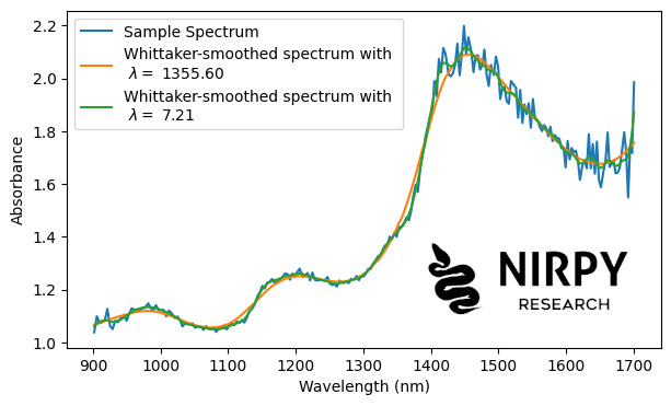
As you can see, I calculated two versions of the smoothed spectra. The first using the “optimal \lambda” as obtained by the curvature method. This value is clearly over-smoothing the spectrum (see the orange curve above), since it is broadening all the main peaks. A much better result is obtained by taking the logarithm of the “optimal value” (green curve), which produces a much better fit to the spectrum, while removing most of the noise.
I believe that the cause of this issue is the fact that the noise level is not the same across the spectrum. Looking at the raw spectrum (blue line), you’ll see that the noise noticeably increases after 1400 nm. The result of the L-curve method (\lambda = 1355.6) produces a good smoothing of the curve after 1400 nm, but it definitely over-smooths it before that. The result using the more conservative \lambda = 7.21 is a much better fit of the spectrum before 1400 nm, and leaves some residual noise after that.
Looking ahead
There are so many ideas that can still be explored using the Whittaker smoothing formalism, and I plan to write more about these topics in the future. A few examples for future posts are:
- How can we optimise the smoothing kernel, or its application, to account for non-uniform noise across the spectrum? This is discussed in our next post.
- The Tikhonov regularisation approach can also be used to estimate (and correct for) baselines. This is the idea behind the Asymmetric Least Squares (ALS) approach, which I briefly discussed in this post.
- Whittaker smoothing can be incorporated into scikit-learn pipelines as another smoothing filter.
- If you acquire more spectra of the same sample (as I’ve done with the dataset used here), there are ways to estimate the noise statistics, in a way that is not accessible with a single spectrum. How can this information be put to good use to optimise the smoothing filter?
As always, comments and ideas are very much appreciated.
Thanks for reading and until next time!
Daniel
References
[1] Paul H. C. Eilers (2003). A Perfect Smoother, Anal. Chem. 75 (14): 3631–3636.
[2] E. T. Whittaker (1922). On a New Method of Graduation, Proceedings of the Edinburgh Mathematical Society, 41: 63 – 75.
[3] P.C. Hansen, Intro to Inverse Problems, Chapter 5, Lecture notes.
**
The feature image is a photo by the author.