PCA and kernel PCA explained

Principal Components Analysis is arguably one of the most important algorithms used in data preprocessing, in a large number of applications. PCA is a linear algorithm. It essentially amounts to taking a linear combination of the original data in a clever way, which can help bring non-obvious patterns in the data to the fore. In order to deal with the presence of non-linearity in the data, the technique of kernel PCA was developed. While certainly more involved than good old PCA, the kernel version enables dealing with more complex data patterns, which would not be visible under linear transformations alone.

In this tutorial we are going to work through a step-by-step implementation of both PCA and kernel PCA. With this approach, I hope, we should be able to grasp the key concepts pertaining to both algorithms. While we are going to write down both algorithms from scratch, we’ll also compare the results with the scikit-learn implementation of the same algorithms. In this way, we’ll have both a sanity check and a working example for future reference.

Before diving into the tutorial, here’s a few links to other tutorials on this site discussing PCA. There may be a bit of repetition of key concepts, but I trust it will be useful to have this tutorial for reference.

• Introduction to PCA
• Classification of NIR spectra using PCA
• Detecting outliers with PCA

Also, the code used for this tutorial is available as a standalone Jupyter Notebook on Github.

A final thing: if you enjoy reading this content, and you find it useful, please consider supporting the blog on Patreon. Supporters have access to additional material and participate to our patron-only Discord community. Thank you.

Principal Component Analysis

Skimming through search engine results for “Principal Components Analysis” or “PCA” you’ll find different definitions or characterisations of the PCA algorithm. One of the most common of these is dimensionality reduction. Somewhat more dramatically, the same concept is expressed by saying that PCA is used to reduce the curse of dimensionality. Or, in a more neutral tone, PCA is described to be an unsupervised decomposition algorithm.

So, what do all these things actually mean when it comes to machine learning or regression applied to spectral data?

Let’s begin with this dimensionality reduction business. What does it mean that PCA is used for dimensionality reduction? To understand this concept let’s start with a geometrical example.

Consider a surface, such as the one drawn in the picture below. Suppose now that we are going to draw the projection of this surface onto a horizontal plane. To keep track of the elevation of the surface, we colour code the plane projection as a contour plot. Blue means low elevation, red means high elevation, and all the shades in between.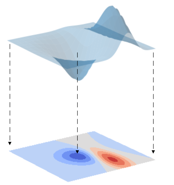

What we accomplished with this operation is the reduction of the geometrical dimensionality of our data. We went from a surface in a three-dimensional space to a projection onto a two-dimensional plane. And in this process, we didn’t lose any of the information content of our data. In other words, we can now fully describe our data on a plane rather than in a 3D space.

This is the key idea of Principal Components Analysis: trying to reduce the number of variables in our data without losing (too much of) the information originally present in our data.

Dimensionality of a spectrum

Now, if you are familiar with spectroscopy you can ask yourself: Hang on a second, what is the dimensionality of a spectrum?  Isn’t a spectrum simply a one-dimensional dataset, for instance absorbance or reflectance as a function of wavelength (or wave number, or energy)?

OK, here’s the trick: instead of considering the wavelength as a continuous variable, as you would do mathematically, we consider each and every wavelength as a separate variable (which we really should be doing since we have a discrete array of wavelengths). Hence, if we have N wavelengths, our spectrum can be considered as a N-dimensional function in this multi-dimensional space.

And here is the advantage of using Principal Components Analysis. PCA will help reduce the number of dimensions of our spectrum from N to a much smaller number.

Before working through the code however, I need to make an admission. In the example of the surface that I’ve shown before… well I cheated a little bit. Some amongst you may have noticed already. I claimed that we’ve reduced the geometrical dimensionality of the data (from 3D to 2D on a plane), which is true, but in the process we added another dimension. We added the colour!

We swapped one geometrical dimension (the elevation of the surface) for another kind of variable, the colour code of the graph. So in total we haven’t reduced the total number of dimensions used to describe the data. We have the same number of variables as we had before.

The aim of the surface example was good to get the discussion going and grasp the essence of PCA. But it was not technically correct. So, let’s forget about the surface from now on, and move on with some real-world examples.

Dimensionality reduction and PCA algorithm

We are finally ready to write some code. We are going to decompose NIR spectral data from fresh plums. The data is available for download on our Github repo.

Here’s the list of imports we’ll need today.

Now let’s write down our own PCa function. Here’s the code

Let’s go through this function step by step. The first line runs a standard scaler over the data. The standard scaler normalises the data so that the transformed data has zero mean and standard deviation  equal to one. Now we get into the real PCA algorithm. We mentioned that PCA is a linear transformation of variables. PCA takes the N coordinates of our spectrum (think of N axes in a N-dimensional space if that is your thing) and finds a transformation of variables into a new set of (initially) N other axes. Amongst the countless ways this can be done, PCA selects the first axis in the new coordinates to be the one that maximises the variance of the data (when projected onto it). The second axis will be the one that will produce the second-highest variance, and so on.

Here’s a picture from one of our previous posts in which the red arrow represents the direction of maximal variance for 2-dimensional data. In this simple example PCA would roughly correspond to a rotation of the axes so that the first axis will coincide with the direction of the red arrow. 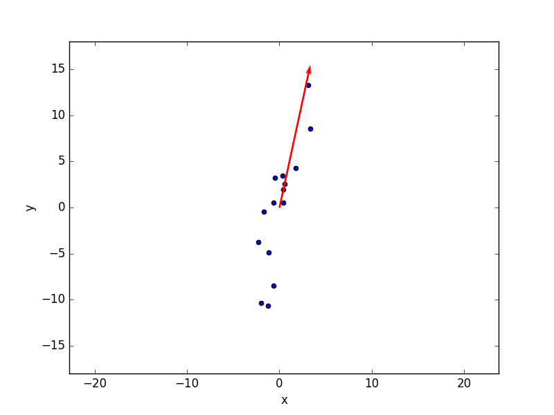This operation is accomplished mathematically (check the code above) by calculating the eigenvalues and eigenvectors of the covariance matrix of our data. The eigenvectors are the new directions in the N-dimensional space (the new axes) and they are sorted in order of decreasing value of the corresponding eigenvalue.

In the code above there is an additional step, which flips the eigenvectors so that they have a deterministic direction. This line is taken straight from the corresponding implementation done in scikit-learn. It is not, strictly speaking, required, but it circumvents the ambiguity that may arise in the direction of the eigenvectors. Referring again to the 2D case in the figure above, the red arrow is drawn pointing up. However an admissible solution will be the same with the red arrow pointing down. Both solutions define the same axis with a directional ambiguity. Flipping the eigenvectors sign in a repeatable manner will avoid that problem.

OK, finally, the PCA decomposition is obtained by taking the dot product of the data and the eigenvectors matrix. Note that in order to calculate eigenvectors and eigenvalues, we do require the complete set of N components. When building the eigenvector matrix however, we can decide to keep a subset of it (default is 2 in the function above), which accomplishes the dimensionality reduction we were after.

Good, let’s import the data and do a standard scaler (which we are going to use later).

Now let’s run the scikit-learn PCA and our implementation on the same data and compare the results by making scatter plot side by side

As you can see, there’s some minor difference in some of the points around the centre of the plots, but for the rest is pretty good. The differences are more evident for the points whose values are close to zero for both PC1 and PC2, which suggests some numerical difference in the eigenvalue decomposition for low values.

Besides these minor differences, the two algorithms do essentially perform in a similar manner. You can certainly keep using (as I will probably do) the scikit-learn implementation, but  at least you know what is going on under the hood.

Let’s move on to kernel PCA

Kernel PCA

Here’s the catch. The PCA transformations we described above are linear transformations. We never mentioned that out loud, but the process of matrix decomposition into eigenvectors is a linear transformation. In other words, each principal component is a linear combination of the original wavelengths.

Suppose the aim of PCA is to do some classification task on our data. PCA will then be useful if the data are linearly separable. Take a look at the image below. It represents some (totally made up) data points. The data points are coloured according to a (again, totally made up) classification. On the left hand side the two classes are linearly separable. On the right hand side the classification boundary is more complicated, something that may look like a higher order polynomial, a non-linear function at any rate.

Kernel PCA was developed in an effort to help with the classification of data whose decision boundaries are described by non-linear function. The idea is to go to a higher dimension space in which the decision boundary becomes linear.

Here’s an easy argument to understand the process. Suppose the decision boundary is described by a third order polynomial y = a + bx + cx^{2} + dx^{3} . Now, plotting this function in the usual x-y plane will produce a wavy line, something similar to the made-up decision boundary in the right-hand-side picture above. Suppose instead we go to a higher dimensionality space in which the axes are x,x^{2}, x^{3} and y. In this 4D space the third order polynomial becomes a linear function and the decision boundary becomes a hyperplane. So the trick is to find a suitable transformation (up-scaling) of the dimensions to try and recover the linearity of the boundary. In this way the usual PCA decomposition is again suitable.

This is all good but, as always, there’s a catch. A generic non-linear combination of the original variables will have a huge number of new variables which rapidly blows up the computational complexity of the problem. Remember, unlike my (oversimplified) example above, we won’t know the exact combination of non-linear terms we need, hence the large number of combinations that are in principle required.

Let’s try and explain this issue with another simple example. Suppose we have only two wavelengths, call them \lambda_{1} and \lambda_{2}. Now suppose we want to take a generic combination up to the second order of these two variables. the new variable set will then contain the following:  [\lambda_{1}, \lambda_{2}, \lambda_{1}\lambda_{2}, \lambda_{1}^{2}, \lambda_{2}^{2}]. So we went from 2 variables to 5, just by seeking a quadratic combination! Since one in general has tens or hundreds of wavelengths, and would like to consider higher order polynomials, you can get the idea of the large amount of variables that would be required.

Now fortunately there is a solution to this problem, which is commonly referred to as the kernel trick. We’ll just give the flavour as to what is the kernel trick and how we can implement it in Python. If you want to know more details on the maths behind it, please refer to the reference list at the end of this tutorial/

Ok, let’s call \mathbf{x} the original set of n variables, let’s call \phi(\mathbf{x}) the non-linear combination (mapping) of these variables into a m>n dataset. Now we can compute the kernel function \kappa(\mathbf{x}) = \phi(\mathbf{x})\phi^{T}(\mathbf{x}). Note that the kernel function in practice is an array even though we are using a function (continuous) notation. Now, it turns out that the kernel function plays the same role as the covariance matrix did in linear PCA. This means that we can calculate the eigenvalues and eigenvectors of the kernel matrix and these are the new principal components of the m-dimensional space where we mapped our original variables into.

The kernel trick is called this way because the kernel function (matrix) enables us to get to the eigenvalues and eigenvector without actually calculating \phi(\mathbf{x}) explicitly. This is the step that would blow up the number of variables and we can circumvent it using the kernel trick.

There are of course different choices for the kernel matrix. Common ones are the Gaussian kernel or the polynomial kernel. A polynomial kernel would be the right choice for decision boundaries that are polynomial in shape, such as the one we made up in the example above. A Gaussian kernel is a good choice whenever one wants to distinguish data points based on the distance from a common centre (see for instance the example in the dedicated Wikipedia page).

In the code below, we are going to implement the Gaussian kernel, following the very clear example of this post by Sebastian Rashka. Here’s the function

The first line calculates the squared Euclidean distance between each pair of points in the dataset. This matrix is passed on the second line which calculates the Gaussian kernel. This kernel is also called ‘RBF’, which stands for radial-basis function and is one of the default kernels implemented in the scikit version of kernel PCA.

Once we have the kernel, we follow the same procedure as for conventional PCA. Remember the kernel plays the same role as the covariance matrix in linear PCA, therefore we can calculate its eigenvalues and eigenvectors and stack them up to the selected number of components we want to keep.

Here’s the comparison

The agreement between the two is excellent, so that’s encouraging.

Again, the aim of this post was to explain how these algorithms work. Going forward you better keep using the scikit-learn implementation, but you’ll know the exact meaning of the parameters and be able to navigate through the choice of kernel.

Hope you enjoyed this tutorial on PCA and kernel PCA. If you did, please consider supporting the blog on Patreon.

Thanks for reading and until next time,

Daniel

References

• Blog post by Sebastian Rashka
• Technical paper on kernel PCA by Quan Wang