Backward Variable Selection for PLS regression

Variable selection, or specifically wavelength selection, is often a really important intermediate step to develop a good prediction model based on spectroscopic data. If you have been reading these articles this is not news to you: not all wavelength bands have the same predictive power for the primary parameter of interest. It is better therefore to eliminate the bands that are least useful, which often improve the quality and robustness of the model. Today we’ll discuss a band selection method called Backward Variable Selection (or Elimination) and we’ll apply it to PLS regression.

I have discussed a few different flavours of band selection in past articles. You can refer to these posts for some more background information.

• A variable selection method for PLS in Python
• Moving window PLS regression
• Wavelength band selection with simulated annealing

For the topic of today, you can also check a paper by Pierna et al. linked here and cited at the end of this post [1]. The data used for this example are taken from the paper by Ji Wenjun et al. linked here [2], and the associated data is available here.

Backward Selection PLS: a minimal example

The concept underlying Backward Selection PLS is fairly simple.

1. Define you model of choice. In this case, PLS regression;
2. Define a suitable metric. For this example, RMSE in cross-validation;
3. Bin the wavelengths of your data into bands. For the data used here, we start with 210 wavelengths from 310 to 2500 nm. We then bin the wavelengths into groups of 5, ending up with n=42 bands (42×5=210). The importance of this step will become clear as we go.
4. Fit a PLS regression model to the binned dataset including all n bands. Calculate the RMSE-CV. This is going to be our baseline to be compared with.
5. Loop over the bands. Remove one band at a time and fit a PLS model to the remaining n-1 bands. The band that, once eliminated produces the sharpest decrease in the RMSE-CV, is discarded.
6. Repeat the process above with n-1 bands. Loop over them and discard the band that, once eliminated, reduce the RMSE-CV the most.
7. Repeat and repeat, iteratively discarding bands, until you reach a point where the RMSE-CV won’t decrease any longer. That is when you stop iterating as you’ve eliminated all bands that are poorly correlated with the quantity you want to predict.

As you can see, we are discarding bands backwards, one at a time, each time getting rid of the worse performing.

OK, let’s see how this works in practice. For clarity, let’s just show the sequence of commands up to the step 5 of the previous list. In essence we want to show how to eliminate just one variable, to avoid the complication of the double loop for the time being.

Let’s begin with the imports

Now, let’s load the data, apply a Savitzky–Golay smoothing filter and plot the spectra

Now it’s time to bin the data into wavelength bands. As anticipated, we’ll define 42 bands, each containing 5 adjacent wavelengths of the original spectra. A neat trick to do with Numpy is to reshape the original array by adding one dimension and then summing over the added dimension.

Finally, let’s fit a baseline PLS regression model. For this I’m going to use a few utility functions, which are defined at the end of this post. These functions perform basic PLS regression, optimise the number of PLS component to be used in the regression model, and plot the results.

This code will print the following text

and produce this plot.

That is an OK starting point but there ample room for improving our model. Let’s write a script to perform a single variable elimination and explain it step by step. Let’s start with the code.

For simplicity, in this example, we are using the entire dataset for this optimisation. In real cases you may want to split your dataset into a training and test set, and perform the optimisation on the training set only.

Anyway, we first define a list to be populated by the RMSE values to be calculated at each step. Then we define a Leave-One-Out (LOO) cross-validator. Note that however, we are not using the LOO cross-validator for cross-validation of the PLS regression. In a normal cross-validation procedure using LOO you would eliminate one measurement at a time (not one band). Unlike that, we use the LOO as a nifty way to iterate over the wavelength bands, discarding one at a time.  At each step the variable train_wl is the wavelength band that is eliminated. A model is fitted and cross validated without it, and a RMSE-CV (using standard K-fold cross-validation) is calculated.

At the end of the sequence, which here consists of 42 iterations, we can plot the result along with the baseline RMSE-CV:

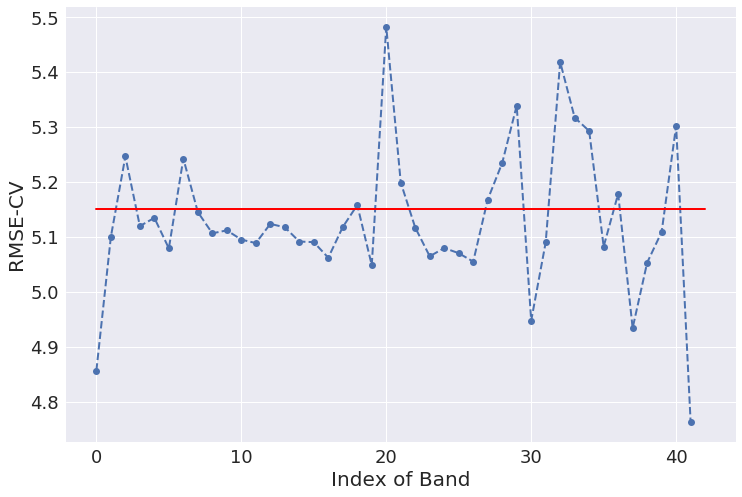
Let’s repeat once again what we have done. First we calculated a PLS model using all bands and estimated the RMSE-CV of such model. That is our baseline (red curve in the chart above). Then we removed one band at a time and each time fitted a new PLS model with the remaining (42-1) bands. For each of these models we estimated the RMSE-CV, which is plotted as blue dots in the graph above.

It’s easy to convince yourself that some of the bands are quite deleterious to the overall model because, once removed, produce a substantial decrease in the RMSE-CV. The the last band, in the instance above, produces the largest improvement once removed. Getting rid of that band would produce an improvement of the RMSE-CV of almost 10%. That is clearly the band we want to eliminate in our bands selection procedure, but we can iterate the process over the remaining band, which is the topic of the next section.

Backward Variable Selection for PLS regression

Now that you understand the basic mechanism, it should be quite easy to iterate over the bands and remove one at a time. The approach used here is to define the arrays to be optimised. One array for the spectra and one for the wavelength bands. Elements will be deleted from these arrays as the optimisation progresses. Let’s call these arrays Xr_optim and wlr_optim with obvious meaning and define them, at the beggining, exactly as we did for the Xr and wlr arrays above. Here’s the full code.

To track the minimisation of the RMSE-CV, we initialise the relevant variable rmscv_min to the baseline value. For each run of the LOO process we remove one band and calculate the minimum of the RMSE-CV of the new model. If this value is less than the previous we keep going, otherwise the loop is interrupted and the optimisation process comes to an end.

While the optimisation is in progress, this code prints the current index of the band being remove, the RMSE-CV and R^2 of the corresponding model. That is overwritten at each step to avoid filling up the available space (The trick is to use stdout.flush() at the end of each iteration). At the end of one LOO loop a line is printed containing the information on the index of repetition, the band that has been deleted and the best values of the RMSE-CV and R^2 attained at that stage.

Running the code above, I got the following output printed on screen.

The improvement is noticeable. If we now run the regression model with the optimised bands, this is what we obtain.

Here you go. A minimal code to run your own Backward Variable Selection for PLS Regression.  Thanks for reading and until next time,

Daniel

References

1. J. Pieran et al., A Backward Variable Selection method for PLS regression (BVSPLS), Analytica Chimica Acta 642, 89-93 (2009).
2. J. Wenjun et al., In Situ Measurement of Some Soil Properties in Paddy Soil Using Visible and Near-Infrared Spectroscopy, PLOS ONE 11, e0159785 (2016).
3. Featured image credit: Valiphoto.

Python functions used in this post