Binary classification of spectra with a single perceptron

The perceptron (sometimes referred to as neuron) is the building block of basic artificial neural networks called feed-forward neural networks. The perceptron is in essence a mathematical function that receives some inputs and produces an output depending on some internal parameter. In this tutorial we are going to introduce the perceptron as a classifier. More specifically we will revisit a problem we already encountered: the classification of spectra belonging to a binary class. In doing so we’ll demystify the concept of perceptron and introduce the all-too-important algorithm of gradient descent.

In a previous post we addressed the problem of binary classification of spectra using PLS Discriminant Analysis. If you haven’t read that post, please take some time to go over it, before working through this one.

PLS-DA is a class of methods that uses partial least squares to solve a classification problem. We have discussed how PLS is naturally derived for regression problems as it outputs real numbers (and not categorical – or integer – variables). It can however be used to reduce the dimensionality of the data set (much like PCA or LDA). Once the dimensionality is reduced, a classification algorithm can be applied on the reduced inputs to predict a categorical variable. In the first tutorial we have accomplished the last task by simply thresholding the output of the PLS. In this tutorial we want to get a tad more sophisticated and use a perceptron instead.

Here’s what we are going to do. First we’ll present a nice and easy introduction to the perceptron as a mathematical concept. Secondly, we are going to describe how to train your perceptron, which will lead us to the gradient descent algorithm. Finally, we are going to bring our data in, and build a spectra classifier using PLS and a single perceptron. There’s some ground to cover, so let’s get going.

The perceptron

If the name sounds like a sci-fi thing of the 1950s, it’s because that’s when the perceptron idea was formalised by Frank Rosenblatt. While its inventor devised the perceptron as an actual device (somehow emulating an actual neuron in the brain), in modern terms the perceptron is in fact a mathematical function. It receives some input and spits out some output. Let’s write that as y = f(x). The input is x and the output is y.

The specific value of the output depends of course on the type of function and the internal parameters of such a function. Such internal parameters are called weights. Let’s look at the simplified picture below to understand how it all works.

Here’s a basic perceptron having two inputs, which we called x_{1} and x_{2}, an open input, which we called b, and an output y. The dangling link is generally referred to as bias of the perceptron. We’ll come back to it later.

The perceptron function is a combination of two mathematical operations.

The first is the dot product of input and weight plus the bias: a = \mathbf{x} \cdot \mathbf{w} + b= x_{1}w_{1} + x_{2}w_{2} +b. This operation yields what is called the activation of the perceptron (we called it a), which is a single numerical value.

The activation is fed into the second function, which is a sigmoid-type function, for instance a logistic or a hyperbolic tangent. Let’s go with a logistic for this example:

The logistic defined above is limited between 0 and 1. It’ll be close to 0 for low values of the activation and close to 1 for higher values. You can see how the sigmoid is leading us towards the binary classifier we are seeking. The transition for 0 to 1 happens smoothly, which can be loosely interpreted as yielding the probability of an output being classified as belonging to either class.

Training the perceptron means adjusting the value of the weights and bias so that the output of the perceptron correctly attributes each sample to the right class. In a supervised classification setting, the parameters are adjusted so that the output from training data is close to the expected value.

Training the perceptron for binary classification of NIR spectra using gradient descent

In keeping with the style of this blog, we won’t be discussing the mathematical subtleties of the gradient descent algorithm used for training. We will however present a simple implementation of gradient descent in Python, which will give you a taste of how many optimisation algorithms work under the hood.

OK, let’s begin as usual by writing the imports and loading a dataset:

The data set for this tutorial consists of a bunch of NIR spectra from samples of milk powder and coconut milk powder. The two were mixed in different proportions and NIR spectra were acquired. The data set is freely available for download in our Github repo..

The data set contains 11 different classes, corresponding to samples going from 100% milk powder to 0% milk powder (that is 100% coconut milk powder) in decrements of 10%. For the sake of running a binary classification, we are going to discard all intermediate mixes and keep only the 100% milk powder and 90% milk powder samples. Here’s the code which follows closely what we’ve done in the PLS-DA post

Having selected two classes, we run a PLS decomposition with two components:

Let’s take a look at the scatter plot of the two latent variables

Vanilla gradient descent

Now it’s time to train the classifier. We are going to start with the simplest, most straightforward version of the gradient descent. This will let us focus on the key aspects of the algorithms. We are then going to add complexity to it, in order to address some of the issues present in the vanilla model.

Firstly we are going to define a handy function to calculate the sigmoid

And this is the training loop implementing gradient descent. First we write the code, then we’ll explain it step by step

The very first step is the Standard Scaler of the inputs. This is not really required here (or in general) but it may be important for reasons that are going to be clear in a little bit.

The second step is initialising the weights. We opted to initialise the weights to a random number between zero and one. Note that the size of the weight array is the same as the number of PLS components. Since we are doing a binary classification, this number is 2.

The third step is to set the values of the numerical parameter required for the gradient descent. This parameter (we called it eta) is commonly known as the learning rate (neural networks require defining the learning rate, with exactly the same meaning).

The iterative loop follows the scheme:

1. Calculate the activation as the dot product of inputs and weights
2. Calculate the output by applying the above-defined sigmoid
3. Calculate the error, by taking the difference between the known variable and the output
4. Calculate the gradient vector, which turns out to be the dot product between the (transposed) inputs and the error
5. “Descend” (that is decrease) the gradient by taking a step in the direction in which the gradient decreases (which in turn means decreasing the error).

The last two steps require a bit of maths to be worked out. I decided not to go over the details of it, to avoid unnecessary complications. The philosophy behind is however simple. In order to decrease a function (in this case the error) we would like to find the “downhill” direction of its gradient. At a first approximation this means: w \rightarrow w - \eta g.

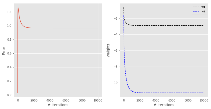
After running the loop for 10,000 iterations, here’s the graphical output

The error is decreasing (it should ideally approach zero). The weights are becoming more and more negative (increasing in magnitude). In order to appreciate how this perceptron will classify our data, we are going to calculate its outputs for values covering the range of our latent variables. In this way we will be able to draw a classification contour overlapped to the scatter plot. Here’s the code:

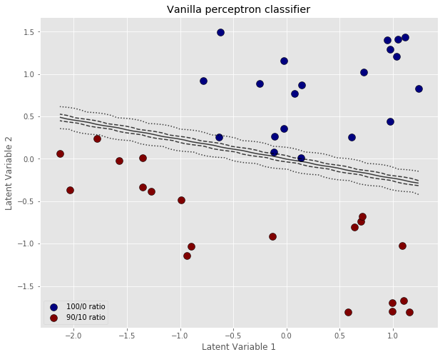
The important thing to notice here, is that the classification boundary of the perceptron is fairly steep, when the perceptron is trained with the vanilla algorithm. You’d expect that increasing the number of iterations will result in an even smaller error, larger and negative weights, and an even steeper classification boundary.

A steep boundary means that a tiny variation around the 50/50 line may result in a different outcome. In other words, ever so slight variations of the inputs can result in the spectrum classification switching from 0 to 1. This sort of instability is another example of “over-fitting” i.e. a prediction model being extremely sensitive to the training data, at the risk of not being able to generalise to test data.

Adding a regularisation parameter

To try and mitigate the problem of over-fitting, the strategy is in general to accept a slightly worse model on the training set, which will result in smaller (in magnitude) weights and a more gradual classification boundary.

In gradient descent, this can be done by adding a penalty \alpha , sometimes called weight decay. This term prevents the weights from becoming too large in magnitude (hence the name “decay”). Here’s the improved gradient descent code (only change is adding a line defining alpha, and regularising the gradient descent step)

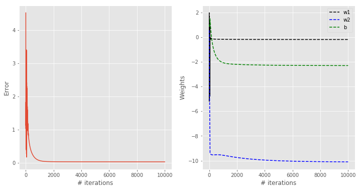
The output of the regularise gradient descent is below.

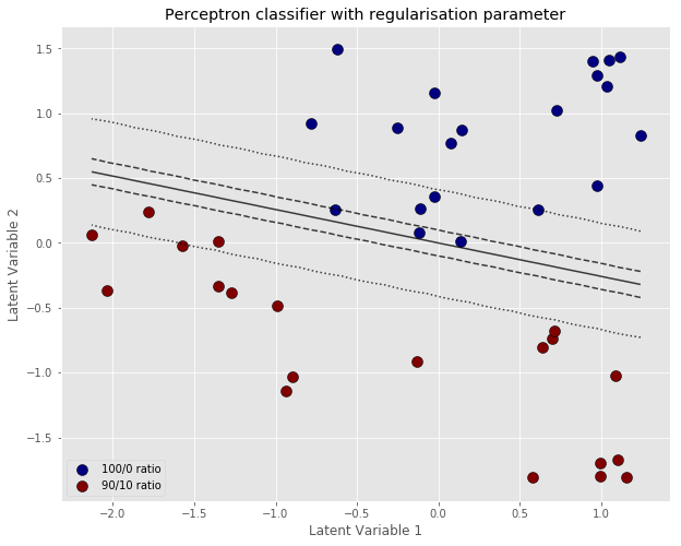
As predicted, the error and the weights do not decrease as much. In fact, the system reaches a steady situation in about 2000 iterations. The classification contour is also wider, which is generally better for generalisation. In other words we are willing to accept a worse performance on this specific data set used for training, which will hopefully result in a more robust model that can generalise better to unknown data.

Adding the bias term

You might have noticed that despite defining the bias, we haven’t in fact coded in the perceptrons we trained so far. A way to add the bias without much changing the code, is to note that the bias can be considered just as another weight, whose input is always fixed to 1. In other words we can include the bias value into the weights array, making sure that we also add a “dummy” latent variable which is identically equal to 1.

This turns out to be better suited to handle scale differences between latent variables. In this specific case the latent variable 1 spans a much larger range than latent variable 2 (see scatter plot at the beginning of this section). This may or may not be an issue (in this case it’s not), and we sidestepped it by scaling the variables to span the same range. Adding the bias term however is a more principled solution to make full use of the parameters at our disposal.

OK, first we are going to redefine our input to include a dummy input column, which is the one associated with the bias input.

And now we can run the gradient descent loop with the relevant changes.

Let’s take a look at the results

You can appreciate how this classification contour looks qualitatively better than the previous results. At the same time, the contour is not too steep, which is good in the sense discussed before.

A few remarks on the gradient descent algorithm

The savvier amongst you may know that Scikit-Learn has already got an implementation of the perceptron, which is in fact a special case of the stochastic gradient descent classification algorithm.

So far we discussed what we simply called ‘gradient descent’, and more precisely must be called batch gradient descent. So, what is the difference between stochastic and batch gradient descent? What are the relative advantages and limitations? Let’s spend a few words on that.

The key difference is in the calculation of the gradient. In our implementations above, we calculated the gradient vector as the dot product of the (transposed) PLS variable vector and the error. The dimensionality of this vector is the same as the variable vector (in our case 2 or 3, considering the bias). However this implies we have to calculate the errors relative to all variables, then compute each component of the gradient, then the dot product. In other words we have to run the entire batch of variables to be able to compute the gradient. The advantage is that, since we have the full gradient, the error is going to deterministically decrease, at least after a few runs (see figures above).

The disadvantage is that the batch may become too large to handle. Data size is not a problem in the simple example described here, but it can become relevant for large data sets and a vast number of variables. Here’s where a trick can be used. Instead of calculating the error on the entire batch of variables, we compute only one component of it (and therefore one component of the gradient). This is obviously much faster. However, since we only picked one direction in this multi-dimensional parameter space, the monotonical decrease of the error is not guaranteed. It will trend down, but not on every step. In this sense this algorithm is stochastic.

Playing around with the scikit-learn perceptron is something we leave for another time. Hope you enjoyed this introductory tutorial to the perceptron. Thanks for reading and until next time,

Daniel