The original post on PLS Regression in Python is still one of the most popular of the entire blog, despite being now a few years old (and despite the presence of many other very good tutorials out there!). Over the years, I’ve received a number of requests for further explanations and for new or improved content, so I finally decided to publish this companion post.
Partial Least Squares (PLS) Regression is one of the mainstays of statistical learning applied to chemometrics. In spite of new and improved methods that have been developed over the years — methods that can often claim improved performances over it — PLS regression is pretty much considered a benchmark, to which one can compare other approaches.
That is, I believe, the reason why my old post still goes very strong, and why I’ve decided to add new material here to complement it. Keep in mind that some of the material presented here already exists elsewhere on this blog (or in the internet ocean), and that large chunks of it can also be applied to other regression techniques. It is however useful, I believe, to have all the content in one place in this post update.
Needless to say: if you haven’t read the original post, feel free to do it now. Here we assume that content to be known. The sections below contains some updated code (compared to the original version) and some additional one, in no particular order. The post is a work in progress, and I will surely add content to it as new ideas will come about.
Optimising the number of latent variables
The original post contains a function, called optimise_pls_cv, that finds the optimal number of latent variables (LV, or components) for a given dataset, where optimal means the number of LV that minimises the root mean squared error (RMSE) in cross-validation. This function can be replaced by a more compact code based on the GridSearchCV function of scikit-learn. Here’s how it works.
First, we write the imports
|
1 2 3 4 5 6 7 8 9 |
import numpy as np import pandas as pd import matplotlib.pyplot as plt from scipy.signal import savgol_filter from sklearn.cross_decomposition import PLSRegression from sklearn.model_selection import cross_val_predict, GridSearchCV from sklearn.metrics import mean_squared_error, r2_score |
Then we load the data and apply the required pre-processing (just second derivative smoothing here, but you can get fancier)
|
1 2 3 4 5 6 7 8 9 10 11 |
# Read data from Github url = 'https://raw.githubusercontent.com/nevernervous78/nirpyresearch/master/data/peach_spectra_brix.csv' data = pd.read_csv(url) # Extract arrays y = data['Brix'].values X = data.drop(['Brix'], axis=1).values wl = np.arange(1100,2300,2) #wavelength # Calculate second derivative X2 = savgol_filter(X, 17, polyorder = 2, deriv=2) |
Finally, use the grid-search procedure to find the optimal number of components using 10-fold cross-validation.
|
1 2 3 4 5 6 7 8 9 10 11 12 |
# Define the parameter space for the search. Just the number of LV here parameters = {'n_components':np.arange(1,20,1)} # Define the grid-search estimator based on PLS regression pls = GridSearchCV(PLSRegression(), parameters, scoring = 'neg_mean_squared_error', verbose=0, cv=10) # Fit the estimator to the data pls.fit(X2, y) # Optional: print the best estimator print(pls.best_estimator_) # Apply the best estimator to calculate a cross-validation predicted variable y_cv = cross_val_predict(pls.best_estimator_, X2, y, cv=10) # Optional: calculate figures of merit rmse, score = np.sqrt(mean_squared_error(y, y_cv)), r2_score(y, y_cv) |
Plotting the results
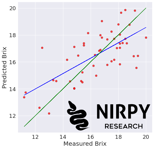
Endless options are available to display the results, but here’s a utility function that produces a scatter plot of measured versus predicted variables, plot a linear fit and a 45 degree line for reference.
|
1 2 3 4 5 6 7 8 9 10 11 12 13 14 15 16 17 18 19 20 |
def regression_plot(y_ref, y_pred, title = None, variable = None): # Regression plot z = np.polyfit(y_ref, y_pred, 1) with plt.style.context(('seaborn')): fig, ax = plt.subplots(figsize=(8, 8)) ax.scatter(y_ref, y_pred, c='red', edgecolors='k', alpha=0.75) ax.plot(y_ref, z[1]+z[0]*y_ref, c='blue', linewidth=1) ax.plot(y_ref, y_ref, color='green', linewidth=1) if title is not None: plt.title(title, fontsize=20) if variable is not None: plt.xlabel('Measured ' + variable, fontsize=20) plt.ylabel('Predicted ' + variable, fontsize=20) plt.xticks(fontsize=18) plt.yticks(fontsize=18) plt.show() |
The function can be applied to the cross-validation data above
|
1 |
regression_plot(y, y_cv, title = "", variable = "Brix") |

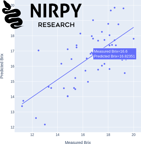
For a more interactive option, Plotly is an excellent place to start.
|
1 2 3 4 |
import plotly.express as px fig = px.scatter(x=y, y=y_cv.flatten(), trendline="ols", width=600, height=600,\ labels = {"x":"Measured Brix", "y":"Predicted Brix"}) fig.show() |

Exporting the data
One option to export the results of the cross-validation process (or any predicted versus actual data in fact) in readable form is to combine the arrays into a pandas data frame and then export to csv file.
|
1 2 |
result_df = pd.DataFrame(np.vstack((y, y_cv.flatten())).T, columns=["Measured", "Predicted"]) result_df.to_csv("export.csv") |
This will give you the option of exporting the data for further processing with different software packages.
Conclusions… but it’s a WIP
As mentioned in the opening, I consider this post as a work in progress. I’m sure there will be many more ideas that I will come up with, or that you, dear reader, will be able to suggest. They will be continually added here.
But for now, thanks for reading and until next time,
Daniel


