This post is the first instalment of a series of posts introducing deep neural networks (DNN) for spectral data regression. In this first post we are going to write some basic code to train a fully-connected DNN using Tensorflow and Keras on sample NIR data. Subsequent posts will deal with parameter optimisation and Convolutional Neural Networks.
The aim of this post is to provide a starting point for students and practitioners to build their own DNN architectures. Plenty of high quality resources are available out there that go above and beyond this introductory tutorial. A few of these resources are listed at the end of the post.
The post is divided into two main blocks. In the first we’ll see a bare-bone DNN scheme. We’ll use this part to explain the meaning of the main parameters used for designing and training DNN, as well as a sample workflow.
In both cases, our aim is to show a practical example, not to provide guidelines on how to select parameters to improve training or prediction. Fine-tuning is something that is very dependent on the data at hand and, besides a few general rules, must be optimised on a case-by-case basis.
The preliminaries
The building block of a DNN is the perceptron (sometimes called neuron). We introduced the perceptron in the context of a classification problem. I recommend you take a look at that post which introduces the concept and the main terms. As discussed there, a perceptron is a mathematical function that takes a bunch of inputs, and generates an output based on the weighted sum of these inputs and a threshold function. The threshold function guarantees that if the weighted sum of the inputs is above a certain threshold, the perceptron will generate an output (the neuron will “fire”). A DNN is a series of concatenated perceptrons.
Training a DNN means finding the values of the weights for each neuron, such that, for any given input, the system generates an output that minimises the error metric for a given training/test dataset. When applied to regression problems – as it will be done here – the DNN is expected to generate a continuous output for any given spectral input, corresponding to the value of the parameter that we wish to estimate through our spectral measurements.
The mathematics of training a neural network (a process called back-propagation) requires some level of knowledge of calculus and discrete mathematics. We are not going to discuss it here, but a few references are added at the end of the post. In practice the back-propagation operations are built in the fitting procedures, so we don’t have to worry about the inner workings of these functions.
OK, let’s begin with the imports (not all of them are needed for this first block; some will be useful later)
|
1 2 3 4 5 6 7 8 9 10 |
import numpy as np import matplotlib.pyplot as plt import pandas as pd from sklearn.metrics import mean_squared_error, r2_score, accuracy_score, mean_absolute_error from sklearn.preprocessing import StandardScaler, MinMaxScaler from sklearn.model_selection import train_test_split import tensorflow as tf from tensorflow.keras import regularizers |
Let’s now load some data. For this post we are going to use data from the paper by Ji Wenjun et al. linked here (see Ref 3). The data available here.
|
1 2 3 4 |
data = pd.read_excel("File_S1.xlsx") X = data.values[1:,8:].astype('float32') y = data["TOC"].values[1:].astype("float32") |
Next, we divide the data into a training and a test set. You can fix the value of the random state to have reproducible splits. Further, we scale the data. Here we use the MinMaxScaler function from scikit-learn, which scales the data between 0 and 1.
|
1 2 3 4 5 6 |
X_train, X_test, y_train, y_test = train_test_split(X, y,test_size=0.4,random_state=79) scaler = MinMaxScaler() scaler.fit(X_train) Xs_train = scaler.transform(X_train) Xs_test = scaler.transform(X_test) |
Deep neural networks: basic architecture
We are now ready to define the DNN architecture. We build a sequential model, where the DNN is a sequence of layers. The layers (and by extension the network) are fully-connected (or dense), which means that each neuron in one layer is connected to all other neurons of the subsequent layer.

|
1 2 3 4 5 6 7 8 |
model = tf.keras.Sequential([ tf.keras.layers.Dense(256, activation='relu'), tf.keras.layers.Dense(128, activation='relu'), tf.keras.layers.Dense(64, activation='relu'), tf.keras.layers.Dense(32, activation='relu'), tf.keras.layers.Dense(16, activation='relu'), tf.keras.layers.Dense(4, activation='relu'), tf.keras.layers.Dense(1, activation="linear")]) |
The first number in the definition of each layer is the number of neurons. The second option defines the activation function, which is the non-linear threshold function we introduced at the beginning of this post, which governs the response of each neuron. The shorthand “relu” refers to a Rectifier Linear Unit which is a function that is zero up to a threshold, and grows linearly afterwards. For the last layer, which is the single output of our model, we use a linear activation function, since the last layer must produce the prediction of the model for each input.
The next step is to compile the model. Compiling the model means assigning parameters to the type of optimisation process we would like to take place during training. For this simple example we specify two parameters: the loss function and the learning rate. The loss function is the error metric we wish to minimise upon training. Here we are going to use the Mean Absolute Error (MAE).
The learning rate refers to the process of training the model using gradient descent. We introduced gradient descent in the perceptron post. The basic idea is that training a neural network is an iterative process of adjusting the weights of each input to each neuron. The adjustment is done by changing the weights in a direction that decreases the gradient function. The step size in the chosen direction is given by the learning rate. A large learning rate means the adjustment will be large. This can lead to fast convergence at the beginning of a training cycle, but can also lead to instabilities when the adjustments required are necessarily smaller, such as towards the end of the training.
The optimal value for the learning rate (as well as for the DNN architecture seen before) generally depends on empirical optimisation. Anyway, the code to compile the model is
|
1 |
model.compile(loss='mean_absolute_error', optimizer=tf.keras.optimizers.Adam(learning_rate=0.0001)) |
Training the model and evaluating its performances
OK, we are now ready to train the network, by fitting the model to the training data and checking the error metric on the test set.
|
1 2 3 |
history = model.fit(Xs_train, y_train, epochs=1000, \ validation_data=(Xs_test, y_test), \ verbose=1) |
An epoch corresponds to one cycle of training whereby all input data is used. Therefore we train the network for a specified number of epochs. We specify the validation data set to be used to evaluate the loss function. Finally, the “verbose” parameter controls the amount of output printed on screen during training (verbose=0 suppresses the output).
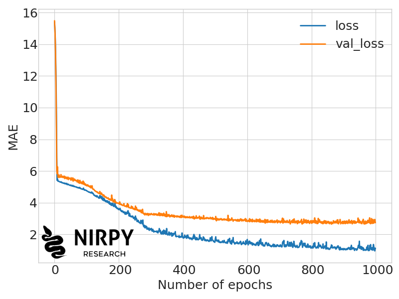
Once the model is trained, we can check how the training has progressed as a function of the number of epochs. In practice we plot the loss function (MAE in this case) for the training and test set respectively.
|
1 2 3 4 5 6 7 8 9 10 11 12 13 14 |
with plt.style.context(('seaborn-whitegrid')): fig, ax = plt.subplots(figsize=(8, 6)) ax.plot(history.history['loss'], linewidth=2, label='loss') ax.plot(history.history['val_loss'], linewidth=2, label='val_loss') plt.xticks(fontsize=18) plt.yticks(fontsize=18) ax.set_xlabel('Number of epochs',fontsize=18) ax.set_ylabel('MAE',fontsize=18) plt.legend(fontsize=18) plt.tight_layout() plt.show() |

The blue line is the MAE on the training set, and the orange line tracks the MAE on the test set. The loss on the training set tends to progressively decrease, albeit at a lower rate with increasing number of epochs. Our objective however is to minimise the MAE on the test set, (i.e. on the data that have not been used to train the model). This is the validation loss, which decreases up to a point and then stays substantially the same.
The gap between training loss and validation loss can be considered a measure of the model overfitting, i.e. the tendency of the model to predict well on the training set, and less so on the test set. A few strategies to reduce the overfitting problem will be discussed in the next post on neural networks.
Before closing, we can take a look at the performance of the model on the test set, by calculating the predictions and the relative metrics.
|
1 2 3 4 |
predictions = model.predict(Xs_test).flatten() rmse, mae, score = np.sqrt(mean_squared_error(y_test, predictions)), \ mean_absolute_error(y_test, predictions), r2_score(y_test, predictions) print("R2: %5.3f, RMSE: %5.3f, MAE: %5.3f" %(score, rmse, mae)) |
which in my case outputs
|
1 |
R2: 0.625, RMSE: 4.086, MAE: 2.738 |
Conclusions and References
Wrapping up, we have a introduced a very simple example of a fully-connected deep neural network for spectral data regression. The aim of this introductory post was to provide a bare-bone code that can be used to explore the use of neural networks when working with spectral data. This is the first post of a short introductory series on training neural networks for chemometrics. In subsequent instalments we’ll see a few techniques to improve the model training and reduce overfitting. Finally, we’ll study a different neural network architecture called Convolutional Neural Network (CNN).
There are a large number of excellent resources out there to learn more about neural networks. Relevant for this post are
- The TensorFlow Python library.
- The Tensorflow regression tutorial.
- F. Chollet, Deep learning with Python, second edition. Simon and Schuster, 2021.
- The dataset is taken from the publicly available data associated with the paper by J. Wenjun, S. Zhou, H. Jingyi, and L Shuo, In Situ Measurement of Some Soil Properties in Paddy Soil Using Visible and Near-Infrared Spectroscopy, PLOS ONE 11, e0159785.
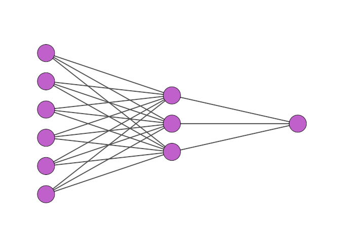
- The featured image has been generated with NN-SVG, a tool created by Alex LeNail. See also A. LeNail, NN-SVG: Publication-Ready Neural Network
Architecture Schematics, Journal of Open Source Software, 4(33), 747.
Thanks for reading and until next time,
Daniel


