Feature selection is one of the topics that come up over and over again when dealing with chemometrics for spectroscopy – and rightly so. In many cases “feature” selection amounts to wavelength (or wavelength bands) selection prior to the regression, to boost the performance of the model. The interesting question is how to search for the best features. Today we discuss a widely used class of algorithms for random search optimisation, called greedy algorithms. To make things interesting, we are going to discuss a kind of feature selection that you might not see very often: principal component selection. The basic idea is to calculate principal components in the usual way, then use a greedy algorithm to find the combination of principal components that yields the best principal component regression model.
For those interested in the topic, we discussed wavelength selection in two examples in previous posts:
Unlike our previous forays in the topic of feature selection, in this and a subsequent post we’d like to take a more general look at algorithmic ways to select features. Feature selection algorithms are a special case of an optimisation algorithm based on a (more or less) random search over the feature space (technically ‘biased’ random walks). Therefore it makes sense to discuss in detail basic algorithms to run such a random search in the best way to optimise the performance of a model.
Everything will become more clear as we progress, but for now let’s define what we mean:
- Optimising the performance of a model means minimising an aptly chosen metric (also called cost, or loss, function). In regression problems the Root Mean Squared Error in prediction or cross-validation are usually valid metrics.
- An optimisation algorithm is a search algorithm over the possible combinations of features that, when used in a regression problem, minimises the cost function.
A straightforward example we discussed in a previous post is to exclude those wavelengths that are poorly correlated with the parameter of interest, thus increasing the overall performance of a model. The concept is however a lot more general. In fact we are going to show an example of an optimisation algorithm used not on primary wavelengths, but on principal components which are derived from those wavelengths. But let’s not rush ahead and go step by step.
The plan for this post is as follows:
-
- We’ll give a gentle but general introduction to the concept of optimisation problems and introduce a basic class of random search algorithms known as greedy algorithms
- We’ll talk specifically of how we can implement a greedy algorithm for principal component selection in NIR spectroscopy
- We’ll discuss common pitfalls of greedy algorithms, which will pave the way to a subsequent post on random search algorithms
Optimisation Problems and Greedy Algorithms
A greedy algorithm is a common approach used to solve an optimisation problem. An optimisation problem is a very wide definition encompassing all those situations that can be recast as a maximisation or minimisation of some metric, or cost function. If you are looking for the best deal for a pair of sneakers, you are trying to solve an optimisation problem. This problem will different depending on your choice of cost function. For instance you may want to find the cheapest sneakers on the market, or given some constraint, for instance a specific brand, what is the best product that satisfies your requirements.
The features we have just described are the two general characteristics of an optimisation problem:
- Having a defined function to maximise or minimise. A cost (or loss) function is usually something you want to minimise (in line with the meaning of “cost” as something you pay)
- Possibly, but not necessarily, having a set of constraints.
Our prototypical situation is to minimise the RMSE of a regression model in a way that may or may not be subject to constraints. In what follows we assume the optimisation problem is in fact a minimisation problem of a cost function. Everything we’ll discuss can obviously be applied to a maximisation problem just as well, with trivial adjustments.
Very well. Now that the definition of optimisation problem is out of the way, let’s discuss greedy algorithms as a class of approaches to iteratively solve the optimisation problem.
First of all, why is the algorithm called greedy? As bad as it might sound, that is just a technical name describing the defining feature of this approach. A greedy algorithm is an iterative optimisation procedure aiming at decreasing the cost function at every step. It essentially amounts to an iterative process in which, at every step, we randomly change the input parameters and evaluate the cost function. If the cost function has decreased we keep the new parameters, otherwise we reset the parameters to the previous step.
Before looking at the details of how to write a greedy algorithm in Python, let’s discuss the regression problem at hand.
Components selection in Principal Components Regression
Principal Components Regression is a linear regression algorithm done on the principal components of a primary dataset. As we discussed in a dedicated post on the topic, a simple linear regression can’t be applied to spectral data because of multicollinearity problems. That is, the signal corresponding to different wavelengths may be highly correlated and this creates serious issues to the least square regression problem based on matrix inversion.
The solution to this problem is to run the linear regression on suitable components extracted from the primary wavelengths. Principal components are an obvious example. Another example – possibly the most widely used of all – is Partial Least Squares (PLS) regression, where the regression is done on the latent variables.
We discussed the advantages of PLS over PCR in this post. This however is not the end of the story. Developing algorithms based on PCR can afford us some flexibility that is not present with PLS. In conventional PCR we just select the first few principal components. The number of principal components to retain is decided on the basis of a cross-validation process. Nobody prevents us however from picking a different set of principal components, not necessarily in order.
Remember that the principal components are calculated according to the spectra only. The primary values (y) do not enter in the PCA algorithm. Therefore the larger principal components are not necessarily the ones that correlate better with the primary values. Therefore, picking and choosing principal components makes the algorithm a lot more flexible and generally improves the result.
That’s all good. The next question however is how do we pick the principal components that give the best regression performances? Here’s where we can use an optimisation algorithm based on random search.
Time to write some code.
Baseline PCR
We are going to use NIR spectra from fresh peaches and corresponding brix values. The dataset is available for download at our Github repo.
|
1 2 3 4 5 6 7 8 9 10 11 12 13 |
import numpy as np import matplotlib.pyplot as plt import pandas as pd from sklearn.decomposition import PCA from sklearn.preprocessing import StandardScaler from sklearn import linear_model from sklearn.model_selection import cross_val_predict from sklearn.metrics import mean_squared_error, r2_score data = pd.read_csv('../data/peach_spectra+brixvalues.csv') y = data['Brix'].values X = data.values[:,1:] |
We will use two basic functions for PCR called (of course) pcr and pcr_optimise_components. Similar functions have been discussed in our PCR post.
|
1 2 3 4 5 6 7 8 9 10 11 12 13 14 15 16 17 18 19 20 21 22 23 24 25 26 27 28 29 30 31 32 33 34 35 36 37 38 39 40 41 42 43 44 45 |
def pcr(X,y, pc): # Run PCA and select the first pc components pca = PCA() Xreg = pca.fit_transform(X)[:,:pc] # Create linear regression object regr = linear_model.LinearRegression() # Fit regr.fit(Xreg, y) # Calibration y_c = regr.predict(Xreg) # Cross-validation y_cv = cross_val_predict(regr, Xreg, y, cv=5) # Calculate scores for calibration and cross-validation score_c = r2_score(y, y_c) score_cv = r2_score(y, y_cv) # Calculate mean square error for calibration and cross validation rmse_c = np.sqrt(mean_squared_error(y, y_c)) rmse_cv = np.sqrt(mean_squared_error(y, y_cv)) return(y_cv, score_c, score_cv, rmse_c, rmse_cv) def pcr_optimise_components(Xpca, y, npc): rmsecv = np.zeros(npc) for i in range(1,npc+1,1): Xreg = Xpca[:,:i] # Create linear regression object regr = linear_model.LinearRegression() # Fit regr.fit(Xreg, y) # Cross-validation y_cv = cross_val_predict(regr, Xreg, y, cv=5) # Calculate R2 score score_cv = r2_score(y, y_cv) # Calculate RMSE rmsecv[i-1] = np.sqrt(mean_squared_error(y, y_cv)) # Find the minimum of the RMSE and its location opt_comp, rmsecv_min = np.argmin(rmsecv), rmsecv[np.argmin(rmsecv)] return (opt_comp+1, rmsecv_min) |
The function pcris a simple cross-validation PCR with a set number of principal components. It makes use of the cross_val_predict function of scikit-learn to return the predicted values and a bunch of metrics.
The function pcr_optimise_components is instead used to find the optimal number of principal components by minimising the RMSE in cross-validation. This is done by adding principal components one by one and calculating the corresponding RMSE.
The following code is a basic PCR regression making use of the two functions above.
|
1 2 3 4 5 6 7 8 9 10 11 12 13 14 15 16 17 18 19 20 |
pca = PCA() Xpca = pca.fit_transform(X) opt_comp, rmsecv_min = pcr_optimise_components(Xpca, y, 30) predicted, r2r, r2cv, rmser, rmscv = pcr(X,y, pc=opt_comp) print("PCR optimised values:") print(" R2: %5.3f, RMSE: %5.3f"%(r2cv, rmscv)) print(" Number of Principal Components: "+str(opt_comp)) # Regression plot z = np.polyfit(y, predicted, 1) with plt.style.context(('ggplot')): fig, ax = plt.subplots(figsize=(9, 5)) ax.scatter(y, predicted, c='red', edgecolors='k') ax.plot(y, z[1]+z[0]*y, c='blue', linewidth=1) ax.plot(y, y, color='green', linewidth=1) plt.title('Conventional PCR') plt.xlabel('Measured $^{\circ}$Brix') plt.ylabel('Predicted $^{\circ}$Brix') plt.show() |
The code prints the following output
|
1 2 3 |
PCR optimised values: R2: 0.546, RMSE: 1.455 Number of Principal Components: 19 |
And this is the scatter plot:

Principal component selection with a greedy algorithm
The result of the conventional PCR is not exciting. The simple algorithm written in the pcr_optimise_components function does not allow for a free selection of principal components. It only allows selecting the first n principal components in the order they are produced by PCA.
Suppose instead we’d like to find the optimal choice of 15 principal components out of 30. Optimal means the combination of principal components that minimises the RMSE in cross-validation. Working this problem into a greedy optimisation can be done in the following way:
- Start with a random selection of 15 principal components out of 30
- Create two lists: one with the selected principal components and one with the excluded principal components
- Use the
pcr_optimise_componentsto find the best RMSE in this configuration - Swap a random element of the first list with a random element of the second list
- Find the best RMSE in the new configuration
- If the new RMSE is smaller than the previous, keep the new configuration
- Repeat 4-6 a few hundred times or until convergence
Here is the Python code to accomplish the algorithm above. Note this code assumes the PCA decomposition has been already done, see previous code snippet.
|
1 2 3 4 5 6 7 8 9 10 11 12 13 14 15 16 17 18 19 20 21 22 23 24 25 26 27 28 29 30 31 32 33 34 35 36 37 38 39 40 41 |
tot_pc = 30 #total number of PCs sel_pc = 15 #number of PCs we want to select # Generate random sample to start with p = np.arange(tot_pc) np.random.shuffle(p) pc = p[:sel_pc] # Selected Principal Components notpc = p[sel_pc:] # Excluded Principal Components Xop = Xpca[:,pc] # Selected PCA-transformed data # Out of this random selection, choose the first n PCs that optimise the RMSE in CV opt_comp, rmsecv_min = pcr_optimise_components(Xop,y,tot_pc) print('start',opt_comp, rmsecv_min) # Greedy algorithm for i in range(500): # Make a copy of the original lists on PCs new_pc = np.copy(pc) new_notpc = np.copy(notpc) # Swap two elements at random between the copied lists r1, r2 = np.random.randint(sel_pc),np.random.randint(tot_pc-sel_pc) el1, el2 = new_pc[r1],new_notpc[r2] new_pc[r1] = el2 new_notpc[r2] = el1 # Select the new PCA-transformed data Xop = Xpca[:,new_pc] # Pick the first n PCs that optimise the RMSE in CV opt_comp_new, rmsecv_min_new = pcr_optimise_components(Xop,y,tot_pc) # If the new RMSE is less than the previous, keep the new selection if (rmsecv_min_new < rmsecv_min): pc = new_pc notpc = new_notpc opt_comp = opt_comp_new rmsecv_min = rmsecv_min_new print(i, opt_comp_new, rmsecv_min_new) print(pc) print('Done') |
After running the iterative optimisation above, we can use the following code to evaluate the result of PCR regression with the selected principal components
|
1 2 3 4 5 6 7 8 9 10 11 12 13 14 15 16 17 18 19 20 21 22 23 24 25 26 27 28 29 |
Xop = Xpca[:,pc] Xreg = Xop[:,:opt_comp] # Create linear regression object regr = linear_model.LinearRegression() # Fit regr.fit(Xreg, y) # Cross-validation y_cv = cross_val_predict(regr, Xreg, y, cv=5) # Calculate R2 score in cross-validation score_cv = r2_score(y, y_cv) # Calculate RMSE in cross validation rmsecv = np.sqrt(mean_squared_error(y, y_cv)) print("PCR optimised values after selection by greedy algorithm:") print(" R2: %5.3f, RMSE: %5.3f"%(score_cv, rmsecv)) print(" Number of Principal Components: "+str(opt_comp)) # Regression plot z = np.polyfit(y, y_cv, 1) with plt.style.context(('ggplot')): fig, ax = plt.subplots(figsize=(9, 5)) ax.scatter(y, y_cv, c='red', edgecolors='k') ax.plot(y, z[1]+z[0]*y, c='blue', linewidth=1) ax.plot(y, y, color='green', linewidth=1) plt.title('PC selection by greedy algorithm') plt.xlabel('Measured $^{\circ}$Brix') plt.ylabel('Predicted $^{\circ}$Brix') plt.show() |
which prints
|
1 2 3 |
PCR optimised values after selection by greedy algorithm: R2: 0.672, RMSE: 1.235 Number of Principal Components: 13 |
And plots
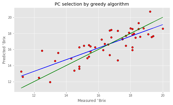
Note that your result may be different from this since each run of the algorithm will start from a different random selection of principal components. In fact, I have decided to use 500 repetition to make sure that different runs produce not too dissimilar results.
As you can see, the improvement is noticeable. We’ve got a nearly 20% improvement in the RMSE, and this result is achieved by using a lower number of principal components altogether.
So this is certainly a very good result. The next question however is: can we do any better? In other words, how do we know if the result found by a greedy algorithm is optimal? (Hint: we don’t). This leads us to the last section of this post.
Properties and pitfalls of greedy algorithms
As mentioned above, a greedy algorithm is such that only changes that decrease the cost function are retained. Since we generally ignore the cost function landscape, we are never sure that the solution found by a greedy algorithm is optimal.
This is best explained using a visual example. Suppose you have a function as the one plotted below, which has two minima. The lowest one is what we call a ‘global minimum’, i.e. is the overall minimum point of the function. We have however also a ‘local minimum’ which is a point that sits below all of its neighbours, within a defined distance.

Now, suppose we would like to find the minimum of this function using a greedy algorithm. What we would do is to choose a random starting point and then move by one step in a random direction. At each point we can evaluate the function so that if we find a lower value we stay in the new position, otherwise we step back to the previous position (this is the sense of ‘biased’ random walk).
This process may well find the global minimum but chances are that it may get stuck in the secondary minimum instead. It is conceivable that the random starting point happens to be close to the secondary minimum and the greedy algorithm will take us all the way down the local minimum. Once there, there’s no chance we can get out, as any step will yield a higher function value and will thus be rejected.
Remember: the algorithm doesn’t don’t know the specific shape of the function, so it blindly takes steps trying to minimise the value. Therefore, we are never sure the solution found by the greedy algorithm is optimal.
In this simple example, we are using a function of two variables only, which allow us to visually explain the problem. In regression problems such as the one discussed above, the RMSE is a function of a large number of principal components. Given the complexity of the function, there will likely be a large number of local minima (let alone the presence of noise). As a consequence each run of the algorithm will likely produce a different result and there is no guarantee the result is the global minimum. Basically we can hope we found a global minimum, or a place sufficiently close to it, allowing for the unavoidable noise in the data.
The take-home message however is that we can’t be certain of hitting a global minimum using a greedy algorithm. In the next post we’ll discuss a modification of the basic greedy approach which enables jumping out of local minima.
Thanks for reading and until next time,
Daniel