Wavelet denoising is an approach based on the wavelet transform. The wavelet transform is a type of signal decomposition similar, in spirit, to the Fourier transform, but with some important differences. In this post, we are going to introduce the concept of wavelet decomposition, and describe how it can be applied for denoising of spectra. If you are not familiar with the concept of denoising, feel free to look at some of our previous posts on the topic, namely:
- Savitzky–Golay smoothing method
- Choosing the optimal parameters for a Savitzky–Golay smoothing filter
- Fourier spectral smoothing method
Otherwise, let’s get started!
Wavelets
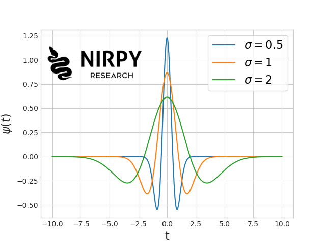
Now, before discussing the wavelets, let’s quickly recap the concept of Fourier transform, which may be more familiar. The Fourier transform is a type of signal decomposition method, which breaks down an analytical signal into combination of sine and cosine functions. In the language of linear algebra, any signal can be written as a linear combination (technically an integral) of (infinitely) many sines and cosines. These functions are chosen as to have increasing frequency, for instance \sin(t), \, \sin(2t), \, \sin(3t), etc. so that the coefficient of the decomposition give information on the different frequency components of each signal. In most cases of physical measurements (such as spectroscopy), the actual signal tends to be more concentrated towards the lower frequencies, while the noise can exist at all frequencies (white noise) or in general to extend to higher frequencies than the signal. Therefore, smoothing a signal with a Fourier method means filtering out the higher frequency components, and retaining the lower frequency components (once again, take a look at our previous Fourier spectral smoothing method post for the fine details). One of the problem of decomposing a signal with harmonic functions, is that these harmonic functions have infinite extension. Take \sin(t) for instance. It exists for every value of the variable t. This means that the corresponding component in Fourier space will be related to all components of the signal, regardless of their time coordinate t. As a consequence, when filtering out high frequency components, we necessarily affect the entire signal. If the discrimination of the signal versus the noise is good enough based on the frequency content, Fourier filtering is perfectly fine. However, one might also look for a decomposition that breaks down the signal into functions that have a finite extent. Wavelets are such functions. Wavelets are oscillatory functions that start at zero, make one or more oscillations, and than return to zero. Take for instance the Ricker wavelet, defined as the second derivative of the Gaussian function: \psi(t) = \frac{2}{\sqrt{3\sigma}\pi^{1/4}} \left(1 - \left(\frac{t}{\sigma}\right)^2 \right) e^{-\frac{t^2}{2\sigma^2}} whose graph looks like this, for different values of \sigma  This is a good example to explain the properties of a wavelet.
- It has a finite extent, i.e. it is non-zero only on a finite interval.
- Its extent can be scaled according to a parameter. In the example above, \sigma controls the extent of the wavelet, whereby smaller \sigma means a more localised wavelet.
- It can be shifted. It is not shown in the graph above, but replacing t with t - t_{0} will shift the wavelet on the horizontal axis by the amount t_{0}.
Wavelet decomposition
Wavelet decomposition is the exact analogue of Fourier decomposition. As we have seen above, a Fourier decomposition computes how much of a signal is described by simple oscillations of increasing frequency: \sin(t), \, \sin(2t), \, \sin(3t), etc. Mathematically, this is described by a convolution. Since wavelets can be scaled and shifted, we can built convolution integrals for wavelets and therefore compute how much of a signal can be described by each scaled wavelet. Moreover, since the extent of the wavelets is finite, we can make that computation at each value of the variable t. I won’t go into the gory mathematical details of the wavelet decomposition. Suffices to say that we want to implement a multi-resolution signal decomposition, first proposed by Mallat that goes like this. A signal has different levels at which it varies. For instance a spectrum might have a very slowly-varying baseline, a slowly-varying signal, faster-varying signal, and high-resolution noise. Normally we acquire the spectrum at the highest resolution possible, to make sure we acquire the faster-varying signal correctly. once acquired however, we can decompose the signal back into the levels at which it varies. Through multi-resolution analysis, a signal is decomposed in a very coarse approximation, and a number of details at increasing level of resolution. Mallat showed that this can be accomplished with a wavelet decomposition. We’ll work through an example using the PyWavelet library available in Python. The basic usage is very simple. We decompose a signal X into coefficients by:
|
1 2 |
import pywt coeffs = pywt.wavedec(X, 'db1', level = 6) |
Here we have used a specific type of wavelet indicated by the string ‘db1’ (these are called Daubechies wavelets), up to the sixth level. Let’s plot these coefficient for an example NIR spectrum. Import the data first:
|
1 2 3 4 5 6 7 8 |
import pywt import pandas as pd import numpy as np import matplotlib.pyplot as plt data = pd.read_csv("../../data/nir_cucumber.csv") X = data.values[:,4:].astype("float32") wl = data.keys()[4:].astype('float32') |
Let’s now calculate the first derivative of the data, using the direct approach using finite differences (For more info on the following code you can check the relevant section of the Python Programming and Numerical Methods book available online)
|
1 2 3 4 |
# Calculate first derivative X1 = np.zeros((X.shape[0], X.shape[1]-2)) for i in range(1,X.shape[1]-1,1): X1[:,i-1] = (X[:,i+1] - X[:,i-1]) / (wl[i+1] - wl[i-1]) |
We can now calculate and plot the wavelet decomposition of the first derivative spectrum.
|
1 2 3 4 5 6 7 8 9 10 11 12 13 14 15 16 17 18 |
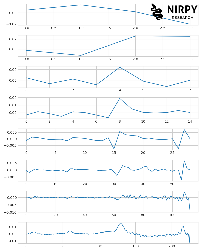
# Wavelet decomposition of the entire set of spectra coeffs = pywt.wavedec(X1, 'db1', level = 6) # Plot the components. The bottom plot is the original spectrum with plt.style.context(('seaborn-whitegrid')): fig, axs = plt.subplots(len(coeffs)+1, 1, sharex=False, figsize=(8,10)) # Remove vertical space between axes fig.subplots_adjust(hspace=0) for i in range(len(coeffs)+1): if i != len(coeffs): axs[i].plot(coeffs[i][0]) # <- we plot only the coefficients of the first spectrum else: axs[i].plot(X1[0,:]) # <- first spectrum plt.tight_layout() plt.show() |
 The original spectrum is in the bottom plot. The coarsest representation of it (its approximation) is in the top plot. The second to the second-last plots represent the increasing levels of detail in the signal. Note how the number of points of each detail increases in moving from top to bottom, while the amplitude of each detail tends to decrease. So, at each successive step of the decomposition, we add a finer detail to the previous one, eventually building up our full signal.
Wavelet denoising: understanding the principle
Now that we have decomposed a signal into its wavelet coefficients, we can also do the opposite operation. Starting from the coefficient we can recover (or “reconstruct”) the original signal. The command for signal reconstruction from coefficients is
|
1 |
X1_rec = pywt.waverec(coeffs, 'db1') |
The wavelet type must match the one used for the decomposition. You can verify, by running the command above, that the reconstructed signal X_rec is identical to the original signal X. This is no surprise as the wavelet decomposition doesn’t discard any information. Smoothing a signal, on the other hand, means discarding some information. Ideally the information to be discarded has to do with the noise distribution and not the signal, but nevertheless we expect the smoothed signal to be different from the original signal. What we can assume, for instance, is that the finest detail, i.e. the one with the finer structure and of smaller amplitude, contains mostly noise. So we can discard it altogether and reconstruct the signal with the remaining coefficients. Now, the finest detail is contained in the last element of the coeffs list. We cannot however just reconstruct the signal by skipping that coefficient. In other words, if we were to run
|
1 |
X_den = pywt.waverec(coeffs[:-1], 'db1') |
we would reconstruct a signal that has a lower resolution than the original one. The correct way of doing this is to preserve the last coefficient, but multiply it by zero (for instance). The code to do that is
|
1 2 3 4 5 6 7 8 9 10 11 12 13 14 15 |
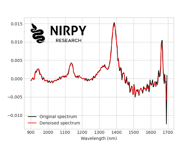
# Make a copy of the coefficients coeffs1 = coeffs.copy() # Set to zero the last coefficient of the copied list coeffs1[-1] = 0*coeffs1[-1] # Reconstruct the signal with the modified coefficients X1_den = pywt.waverec(coeffs1, 'db1') with plt.style.context(('seaborn-whitegrid')): plt.plot(wl[:-2], X1[0,:], 'k', label = "Original spectrum") plt.plot(wl[:-2], X1_den[0,:], 'r', label = "Denoised spectrum") plt.xlabel("Wavelength (nm)") plt.legend(loc='lower left') plt.show() |
Here’s the comparison between the original spectrum (in black) and the denoised spectrum with the crude approach of removing the last coefficient (in red). 
Wavelet denoising with scikit-image
Obviously, if you have been working with data for a while, you can understand why the procedure we have done is very rough. Just deleting one set of coefficients works (sort of) but it doesn’t really account for the specific level of noise in the signal. Luckily for us, a much better wavelet denoising method has been implemented in the scikit-image library, and specifically available here. This library is designed for images, i.e. 2D arrays of data, but the wavelet denoising library does work for 1D data like one of our spectra. This is how we implement it
|
1 2 3 4 5 6 7 8 9 10 11 12 13 14 |
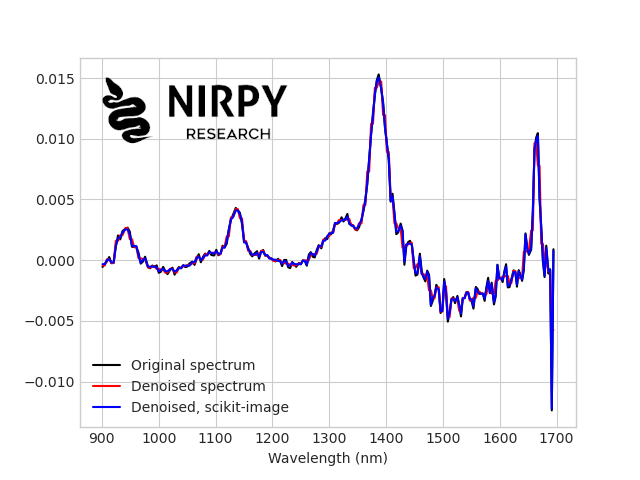
from skimage.restoration import denoise_wavelet X1_den_sk = denoise_wavelet(X1[0,:], wavelet='db1', mode='soft', wavelet_levels=6) with plt.style.context(('seaborn-whitegrid')): plt.plot(wl[:-2], X1[0,:], 'k', label = "Original spectrum") # plt.plot(wl, X_rec[0,:], 'b') plt.plot(wl[:-2], X1_den[0,:], 'r', label = "Denoised spectrum") plt.plot(wl[:-2], X1_den_sk, 'b', label = "Denoised, scikit-image") plt.xlabel("Wavelength (nm)") plt.legend(loc='lower left') plt.show() |
And here’s the comparison with the previous plots  If you zoom in the actual plot (not this image) you’ll be able to appreciate how the last procedure is more optimal. More importantly, by tuning the parameters one can adapt the denoising strategy to the dataset at hand. That’s it for today, and I hope this post gave you some idea to get started with wavelets! Thanks for reading and until next time, Daniel
References
There are a large number of excellent resources out there to learn more about wavelets, wavelet transform, and wavelet decomposition. Relevant resources are
- Shawin Talebi, The wavelet transform
- Book: A Wavelet Tour of Signal Processing, by S. Mallat
- Book: Chemometrics: from basics to wavelet transform, by F-T. Chau et al.


