In 1897, American physicist and inventor Amos Dolbear noted a correlation between the rate of chirp of crickets and the temperature. Crickets would chirp faster the higher the temperature. His paper “The Cricket as a Thermometer” introduced what was later dubbed the Dolbear’s Law.
Besides unveiling this fundamental piece of scientific trivia, this post will use the cricket thermometer to give you an introduction to Principal Component Analysis in Python. We will use the dataset available here relating the number of chirps per second for the striped ground cricket to the temperature in degrees Fahrenheit.
A very gentle introduction to Principal Component Analysis
To keep things simple, we will use these bivariate (that means 2D) data to explain the concept of PCA. If you want a more advanced application of PCA, you can take a look at our post on Classification of macadamia kernels by NIR or Classification of NIR spectra by PCA.
In these other posts we discuss at length on how PCA is used on multivariate data and how it may be a building block to build calibration models for NIR spectroscopy. In fact, using PCA for bivariate data is somewhat excessive, but it helps understanding the basic idea.
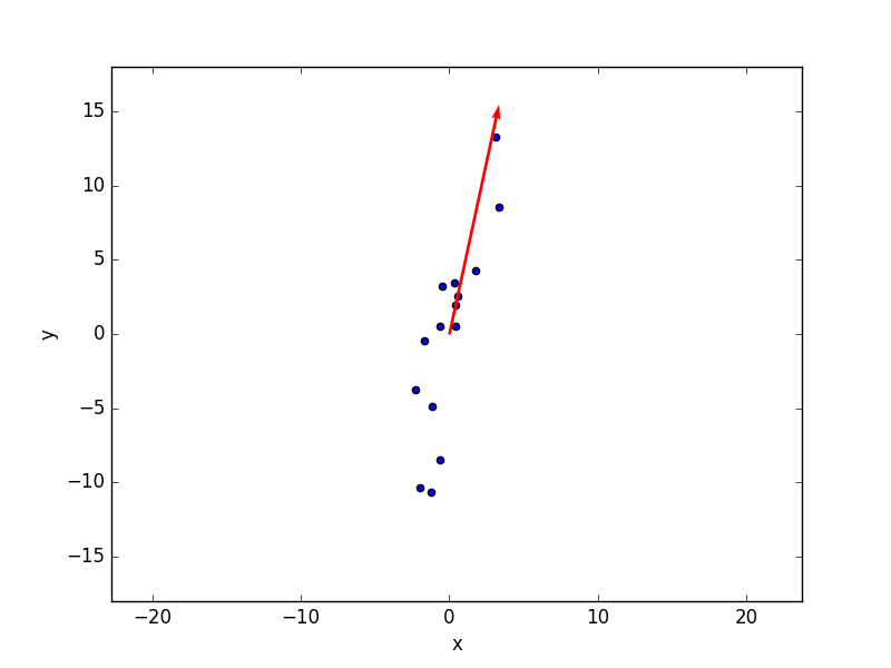
PCA is based on an idea from linear algebra: any vector can be expressed as a linear combination of basis vectors. Since I feel I may be already losing someone, let’s look at the graph of the data: here it is.

The data are charted in an X/Y graph, that means we chose two (conventional) directions over which describe our data. The two axes (actually their directions) are – loosely speaking – the basis we use to calculate the coordinate numerical values.
The axes direction is somewhat arbitrary, that means we can always choose other directions. For instance we could find out the direction over which our data changes more quickly and define that as x-axis. It turns out that the direction over which the data changes the most is the first principal component. PCA is the method that finds and sort main directions over which our data vary.
In our simple 2D example of course we will have only two principal components which, as the conventional x-y axes, will be orthogonal to one another.
Step-by-step PCA algorithm in Python
OK, enough of that, let’s get coding.
|
1 2 3 4 5 6 7 8 9 10 11 12 13 14 15 16 17 18 19 20 21 22 23 24 25 26 27 28 |
import numpy as np import matplotlib.pyplot as plt from pandas import read_csv # Read the data data = read_csv('data.csv') cs = data["X"].values temp = data["Y"].values # Take away the mean x = cs - cs.mean() y = temp - temp.mean() # Group the data into a single matrix datamatrix = np.array([x,y]) # Calculate the covariance matrix covmat = np.cov(datamatrix) # Find eigenvalues and eigenvectors of the covariance matrix w,v = np.linalg.eig(covmat) # Get the index of the largest eigenvalue maxeig = np.argmax(w) # Get the slope of the line passing through the origin and the largest eigenvector m = -v[maxeig, 1]/v[maxeig, 0] line = m*x |
OK, let’s go through the code step by step.
-
- Step 1, reading the data and assigning it to numpy arrays
-
- Step 2, for PCA to work we need to take away the mean from both coordinates, that is we want the data to be centred at the origin of the x-y coordinates
-
- Step 3, group the data in a single array
-
- Step 4, calculate the covariance matrix of this array. Since we are dealing with a 2D dataset (bivariate data), the covariance matrix will be 2×2
-
- Step 5, calculate eigenvalues and eigenvectors of the covariance matrix
-
- Step 6, get the index of the largest eigenvalue. The first principal component we are looking for is the eigenvector corresponding to the largest eigenvalue
-
- Step 7, this one is just needed for plotting. We get the slope of the line that is parallel to the principal component
That’s it! Now we just need to plot the first principal component on top of the data.
|
1 2 3 4 5 6 7 8 9 |
plt.scatter(x, y) plt.xlabel('x') plt.ylabel('y') plt.quiver(0,0, x[0], line[0], units = 'xy', scale = 1, color='r', width = 0.2) plt.axis('equal') plt.ylim((-18,18)) plt.show() |

Done. We found the 2 principal components of our bivariate data, and plotted the largest one on top of our graph. In this simple case, PCA is nothing more than fitting really, but it become very useful when it comes to multivariate data.
PCA the easiest way, and wrap-up
Naturally, nobody expects you to write this many lines every time (well, maybe some of the times) ! The good news is that the scikit-learn Python library will do most of the heavy lifting for you. With just a couple of lines:
|
1 2 3 4 5 6 7 8 |
from sklearn.decomposition import PCA datazip = list(zip(x,y)) pca = PCA(n_components=2) pca.fit(datazip) # Print the eigenvectors print(pca.components_) |
pca_components_ lists the eigenvectors. This is equivalent to the matrix w we found with the step-by-step example, with the only (handy) difference that the eigenvectors are already sorted in decreasing order. That means the principal component is pca_components_[0].
That’s all for this post folks! Hope you enjoyed it. If you’d like to receive regular updates about the content we post, check out our newsletter! Python chemometrics nuggets delivered straight to your inbox!


