At the end of the last post on Whittaker smoothing, I listed a few open issues. One of these issues was how to determine the best regularisation parameter, when dealing with non-uniform noise distribution.
This is the topic of today’s tutorial, but first let’s recap the main results of the last posts:
- We discussed how Tikhonov regularization can be used to perform signal smoothing. This is the approach that we referred to as ‘Whittaker smoothing’.
- Tikhonov regularization is a penalised least-squares approach, whereby a penalty term that depends on the second derivative of the signal is added to the ordinary least squares term. The second-derivative term describe the roughness of the signal we want to minimise.
- The penalty term itself is weighted by the regularisation parameter \lambda , which can be tuned. The larger is the value of \lambda , the stronger the smoothing.
- We introduced the L-curve method as a heuristic method to find the optimal value of \lambda .
A tacit assumption behind the whole discussion was that the signal-to-noise ration (SNR) of the spectrum to be smoothed is constant across the entire wavelength range. In the example we discussed, however, this was not the case. The comparison of the raw spectrum with two smoothed versions of it, was plotted towards the end of last post (and reproduced here).
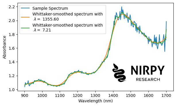

The noise of the raw spectrum (blue line) significantly increases after 1400 nm. We noticed that the result of the L-curve method (\lambda = 1355.6) produced a good smoothing of the curve after 1400 nm, but it definitely over-smoothed it before that. The result using the more conservative \lambda = 7.21 was a much better fit of the spectrum before 1400 nm, but left some residual noise after that.
As noted by Philip Wilson commenting on the previous post, the noise increase after 1400 nm is due to the significant reduction in signal. Here’s an excerpt of Philip’s comments:
A lot of measurements made in the NIR are read noise limited, i.e. the noise on the raw signals is uncorrelated and uniform in magnitude across the spectrum.
[…]
Since transmission signals are ratioed to a baseline measurement (the raw spectrum of the source), and both the sample signal and baseline signal have varying signal levels, the relative effect of a constant noise contribution will vary inversely with the raw signal size. Where the raw signals are small, the transmission noise will be large.
To unpack this concept further, the absorbance spectrum plotted above is obtained by dividing the raw signal by the reference signal. When the intensity of the raw signal is low, the corresponding signal-to-noise ratio (SNR) of the absorbace spectrum increases, which creates the issue observed above.
The better approach, as suggested by Philip, is to smooth the raw signal instead.
In this post we we’ll explore this approach. However (spoiler alert!) we’ll also show that the L-curve method is still producing an over-estimate of the penalty parameter. For this reason we’ll also explore an alternative method, namely Leave One Out Cross-Validation (LOOCV).
That’s a lot to cover… let’s go.
Working with the raw signal
If you haven’t already, take a few minutes to read the previous post on Whittaker smoothing. The code written below is based on that post. Here, I’ll assume that you are familiar with the concepts already explained in the previous post, and focus on discussing the new material.
Let’s start with importing the required libraries and loading a dataset. The dataset is available as a zip file in our GitHub repository. It contains 100 NIR spectra of a Hass avocado. In addition to the absorbance spectra used in the previous post, the dataset contains also the raw signals and the reference spectra. We import these on separate arrays.
|
1 2 3 4 5 6 7 8 9 10 11 12 13 14 15 16 17 18 19 20 21 22 |
import numpy as np import pandas as pd import matplotlib.pyplot as plt import re,glob def natural_sort(l): convert = lambda text: int(text) if text.isdigit() else text.lower() alphanum_key = lambda key: [convert(c) for c in re.split('([0-9]+)', key)] return sorted(l, key=alphanum_key) # Import the data fl = natural_sort(glob.glob("./Avocado_NIR_scans/Avocado_spectra/*csv")) spectra = np.zeros((len(fl), 228)) sample_signal = np.zeros((len(fl), 228)) reference = np.zeros((len(fl), 228)) for i,j in enumerate(fl): df = pd.read_csv(j, skiprows=21) spectra[i,:] = df['Absorbance (AU)'] sample_signal[i,:] = df['Sample Signal (unitless)'] reference[i,:] = df['Reference Signal (unitless)'] wavelength = pd.read_csv(j, skiprows=21)['Wavelength (nm)'] |
Just as we have done in the previous post, we’ll just use the first spectrum of the array to illustrate the smoothing process.
The first thing to note is that the reference signal (i.e. the emission spectrum of the NIR light source) is acquired with a much longer exposure time. This is to make sure that the noise of the reference acquisition is negligible and it won’t affect the spectra, once the reference signal is used to normalise all the acquisitions. The only issue is that the raw data file doesn’t specify the exposure times, so let’s use a rough estimate to plot the data. Let’s assume that the reference signal is captured with 10x longer exposure and plot the comparison.
|
1 2 3 4 5 6 7 |
plt.figure(figsize=(7, 4)) plt.plot(wavelength, sample_signal[0,:], label='Signal') plt.plot(wavelength, reference[0,:]/10, label='Reference') #Divide by 10 to keep the intensity on a similar scale plt.xlabel('Wavelength (nm)') plt.ylabel('Absorbance') plt.legend() plt.show() |
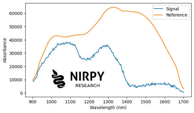
The reference spectrum was divided by 10 so that we can plot it on the same intensity scale as the sample signal. Note also the significant decrease of the signal intensity after 1400 nm.
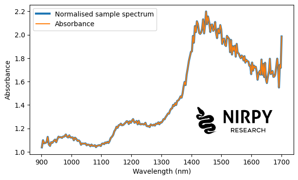
The factor of 10 was not specified in the raw data file, however I verified that it is in fact the correct scaling factor by calculating the normalised absorbance and comparing it to the one provided in the file. There is a perfect match.
|
1 2 3 4 5 6 7 8 |
plt.figure(figsize=(7, 4)) # absorbance = -log(10*signal/reference) plt.plot(wavelength, (-np.log(sample_signal[0,:]) + np.log(reference[0,:]))/np.log(10) , label='Normalised sample spectrum', lw=3) plt.plot(wavelength, spectra[0,:], label='Absorbance') plt.xlabel('Wavelength (nm)') plt.ylabel('Absorbance') plt.legend() plt.show() |
L-curve method applied to the raw signal
Now that we have verified the correct valuefor the ratio of the exposure times between reference and signal, we can get on with the main business of this post.
Focus your attention on the (unnormalised) sample signal two figures above, or more specifically on its noise. You’ll notice that the SNR is approximately the same across the entire wavelength range. Comparing the plot above with the one at the beginning of this post, there is no apparent noise increase after 1400 nm. As noted by Philip Wilson above, the noise increase is an artefact of the normalisation process whereby the signal is divided by the reference spectrum. Working with the raw signal will circumvent this issue.
Let’s follow the same procedure as the previous post, and plot the L-curve for the sample signal.
|
1 2 3 4 5 6 7 8 9 10 11 12 13 14 15 16 17 18 19 20 21 |
signal = sample_signal[0,:] # number of wavelengths n = signal.shape[0] # Second derivative operator D2 = np.diff(np.eye(n), 2, axis=0) # Define the set of lambdas in log scale lambdas = np.logspace(-2,6,1000) rho = np.zeros(len(lambdas)) eta = np.zeros(len(lambdas)) for i, lam in enumerate(lambdas): S_lambda = np.linalg.inv(I + lam * (D2.T @ D2)) x_s = S_lambda @ signal rho[i] = np.linalg.norm(signal - x_s) eta[i] = np.linalg.norm(D2 @ x_s) plt.loglog(rho, eta) plt.xlabel("$ \\rho = || x - x_{s} ||$") plt.ylabel("$ \\eta = ||D_2 x_{s}||$") plt.show() |
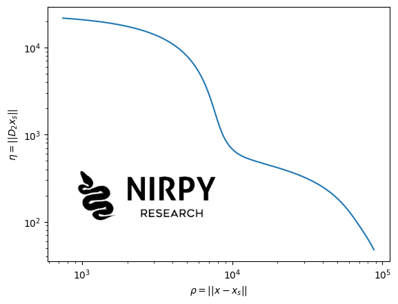
The same considerations made in the previous post apply here. The shape of our curve above is not really like a “L”, unlike other examples you can find online, for instance the (excellent) lecture by Prof. Per Christian Hansen available here [3]. The L-curve you see plotted in slide 14 of the linked lecture, has a very sharp corner, significantly different from the one calculated in our case.
To get briefly ahead of ourselves, I believe this is the reason why the L-curve method is still going to over-estimate the correct \lambda . My conjecture is that the L-curve approach is not sufficiently sensitive: small changes in the curvature of the L-curve correspond to large changes in \lambda .
Nevertheless, let’s complete the procedure. In fact, let’s also modify the relevant function to work with linearly-spaced arrays (as opposed to logarithmic-spaced array used in the previous post) to clear any lingering doubt about the performance of the numerical differentiation. Here’s the function to calculate the position of the knee of the L-curve in linear space.
|
1 2 3 4 5 6 7 8 9 10 11 12 13 14 15 16 17 18 19 20 21 22 23 24 25 |
def l_curve_knee_lin(lambdas, rho, eta): """ Find the corner of the L-curve (max curvature) in linear space. Compare with the corresponding function shown in https://nirpyresearch.com/whittaker-smoothing/ """ rho_hat = np.log(rho) eta_hat = np.log(eta) # First derivatives. d_rho_hat = np.gradient(rho_hat, lambdas) d_eta_hat = np.gradient(eta_hat, lambdas) # Second derivatives dd_rho_hat = np.gradient(d_rho_hat, lambdas) dd_eta_hat = np.gradient(d_eta_hat, lambdas) # curvature formula for a parametric curve (log_rho(t), log_eta(t)) numerator = d_rho_hat * dd_eta_hat - dd_rho_hat * d_eta_hat denominator = (d_rho_hat**2 + d_eta_hat**2) ** 1.5 curvature = 2* numerator / (denominator) knee_loc = np.argmax(np.abs(curvature)) optimal_lambda = lambdas[knee_loc] return curvature, optimal_lambda, knee_loc |
We re-define the array lambdas in linear scale and smooth the signal with the optimal_lambda according to the L-curve method. We also smooth the signal with the logarithm of optimal_lambda, as a comparison.
|
1 2 3 4 5 6 7 8 9 10 11 12 13 14 15 16 17 18 19 20 |
lambdas = np.linspace(1,5000,5000) curvature, optimal_lambda, knee_loc = l_curve_knee_lin(lambdas, rho, eta) # Smoothing kernels S_opt_lambda = np.linalg.inv(I + optimal_lambda * (D2.T @ D2)) S_opt_lambda_mod = np.linalg.inv(I + np.log(optimal_lambda) * (D2.T @ D2)) # Smoothed spectra x_s_opt = S_opt_lambda @ signal x_s_opt_mod = S_opt_lambda_mod @ signal # Plot plt.figure(figsize=(7, 4)) plt.plot(wavelength, signal, label='Sample Spectrum') plt.plot(wavelength, x_s_opt, label="Whittaker smoothing \nwith $ \\lambda =$"+f" {optimal_lambda:.2f}") plt.plot(wavelength, x_s_opt_mod, label="Whittaker smoothing \nwith $ \\lambda =$"+f" {np.log(optimal_lambda):.2f}") plt.xlabel('Wavelength (nm)') plt.ylabel('Signal') plt.legend() plt.show() |
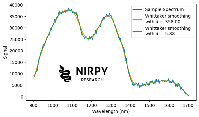
The optimal result of the L-curve method is now (\lambda = 358), which is about 3 times smaller than the corresponding results calculated on the normalised spectra (see plot at the beginning of this post), but it still over-smooths compared to using (\lambda = \ln(358) = 5.88). Hence, working with the raw signal has improved things somehow, since we don’t have to deal with a changing SNR across the spectrum. However, the result of the L-curve method is still larger than what we would expect, likely due to the shape of our L-curve not being very sharp at the “corner” position.
Another method: leave-one-out cross-validation
This is the method first mentioned in the original paper by Eilers [1]. The idea is simple and intuitive, if you have spent some time working on model selection.
- We start from the original spectrum x and we remove the i-th wavelength band, where i is an index running from 1 to N, which is the size of the wavelength array.
- Let’s call x^{(-i)} the spectrum obtained by removing the i-th wavelength band and x_{i} the single value that was removed.
- For a given value of the regularisation parameter, smooth the modified spectrum to get an estimate x_{s}^{(-i)} for the left out point.
- Repeat the above for all points in the spectra and calculate the average squared error
s^{2} = \frac{1}{N} \sum_{1 = 1}^{N} \left( x_{i} - x_{s}^{(-i)} \right)^{2} - The error above depends on \lambda (through x_{s} ), hence you can repeat the procedure by varying \lambda and seeking to minimise s^{2}.
This approach is intuitive, but not parsimonious, for it requires to calculate the Tikhonov regularisation N times for each value of \lambda. Luckily, as mentioned by Eliers [1] (see also [2]), there is a shortcut that doesn’t require these many loops. Without discussing the details, the shortcut is available because the smoothing function is linear (see our previous post):
\hat{x}_{s} = S_{\lambda} x,
where the smoothing kernel is S_{\lambda} = \left(I + \lambda D_{2}^{T} D_{2}\right)^{-1} . In this situation, x_{s}^{(-i)} can be computed from x_{s,i} (the point i of the smoothed spectrum without removing any point) and S_{\lambda, i,i} (the diagonal element (i,i) of the smoothing kernel) without the need of actually removing points and calculating the smoothing over and over. The relevant formula is (see equation (3.18) of [2]):
x_{i} - x_{s}^{(-i)} = \dfrac{x_{i} - x_{s,i}}{1 - S_{\lambda, i,i} },
enabling us to calculate the cross-validation residuals from the standard residuals. The cross-validation sum of squares is then:
CV(\lambda) = \dfrac{1}{N} \sum_{i=1}^{N} \left( \dfrac{x_{i} - x_{s,i}}{1 - S_{\lambda, i,i} } \right)^{2},
The formalism is a bit convoluted, but hopefully things will become clearer by looking at the code for the cross-validation loop.
|
1 2 3 4 5 6 7 8 9 10 11 12 13 14 15 16 17 18 |
lambdas = np.linspace(1,100,100) loocv_sum_squares = [] for lam in lambdas: # Smoothing kernel, function of lambda S_lambda = np.linalg.inv(I + lam * (D2.T @ D2)) # Diagonal of the smoothing kernel S_diag = np.diag(S_lambda) # Smoothed spectrum x_s = S_lambda @ signal # Residuals and error loo_residuals = (signal - x_s) / (1 - S_diag) loocv_sum_squares.append(np.mean(loo_residuals ** 2)) plt.plot(lambdas, loocv_sum_squares) plt.xlabel("$ \\lambda$") plt.ylabel("CV($ \\lambda$)") plt.show() |
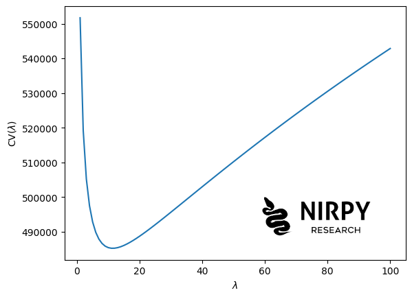
The optimal value of the regularisation parameter using the LOOCV method is
|
1 2 |
min_loc = np.argmin(np.array(loocv_sum_squares)) optimal_lambda = lambdas[min_loc] |
which gives \lambda = 11 for our example. This is a much more reasonable value, not too far from our initial estimate made visually.
Wrapping up: smoothing the signal and converting to absorbance
All is left to do is to apply the optimal regularisation parameter, and then calculate the absorbance, as we did in the first section.
|
1 2 3 4 5 6 7 8 9 10 11 12 13 14 15 16 |
# Smooth signal with optimal lambda S_opt_lambda = np.linalg.inv(I + optimal_lambda * (D2.T @ D2)) S_diag = np.diag(S_lambda) x_opt_s = S_lambda @ signal # Calculate smoothed absorbance smoothed_absorbance = (-np.log(x_opt_s) + np.log(reference[0,:]))/np.log(10) # Comaprison plot with raw absorbance plt.figure(figsize=(7, 4)) plt.plot(wavelength, spectra[0,:], label='Sample spectrum') plt.plot(wavelength, smoothed_absorbance , label='Smoothed spectrum') plt.xlabel('Wavelength (nm)') plt.ylabel('Absorbance') plt.legend() plt.show() |
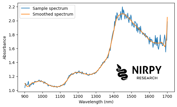
As a final observation, we can confirm that the process of smoothing the raw signal has solved the issue discussed at the start of this tutorial, producing a smooth result also after 1400 nm.
This was a dense blog post, so thanks for reading all the way to the end!
Until next time!
Daniel
References
[1] Paul H. C. Eilers (2003). A Perfect Smoother, Anal. Chem. 75 (14): 3631–3636.
[2] T. Hastie and R. Tibshirani, Generalized Additive Models. Chapman and Hall (1990), pp. 46-47.
[3] P.C. Hansen, Intro to Inverse Problems, Chapter 5, Lecture notes.
**
The feature image is a photo by the author.