The post on Robust PCA sparked a few conversations with readers of this blog on ‘robust’ approaches to data preprocessing. If you worked with real datasets you probably know that a few outliers can really derail your preprocessing pipeline and therefore need to be dealt with appropriately. Robust PCA was an example. A robust version of the Multiplicative Scatter Correction algorithm (Robust MSC), discussed here, is another.
Before working through the code, here’s two references you might want to look at, if you need a refresher on MSC.
- Two scatter correction techniques for NIR spectroscopy in Python
- Include MSC in a custom pipeline using scikit-learn

The wonders of the median
MSC estimates and correct for (undesirable) scattering effects by comparing a spectrum to a reference spectrum. The reference spectrum is assumed to be free of scattering effects.
In practice, a reference spectrum is rarely available. What is more easily available is the average spectrum of a multiple-sample dataset. Assuming that scattering is the results of sample surface effects, and assuming also that these effects vary randomly from sample to sample, the average spectrum should produce a close approximation to a scatter-free spectrum.
However, the average spectrum could be easily affected by the presence of one or more outliers, which then could have a deleterious effect on the rest of the dataset through the MSC correction.
The secret to make a robust version of MSC is surprisingly simple: all we need is to replace the mean with the median. The (arithmetic) mean in a dataset is given by sum of the values divided by their number. The median, instead, is the value that sits exactly in the middle of the distribution. Half of the data points are above the median, the other half sit below.
The median is therefore way more robust against outliers: it makes little difference if a value lies 100 times or 1000 times above the mean. If it falls on the 50% of points on the right-hand side of the distribution, the median won’t change.
This brings us to the promised implementation of a robust version of MSC (RMSC).
Robust MSC correction class
Our implementation of the RMSC follows closely what we’ve done with the custom MSC class developed in a previous post.
RMSC is implemented as a transformer, i.e. a function that modifies the data ‘in a supervised or unsupervised way’ before an estimator (for instance a PLS regressor) can be fitted.
For all the details, refer to the post linked above and to the examples provided in the scikit-learn Github page.
Here’s the class.
|
1 2 3 4 5 6 7 8 9 10 11 12 13 14 15 16 17 18 19 20 21 22 23 24 25 26 27 28 29 30 31 32 33 34 35 36 37 38 39 40 41 42 43 44 45 46 47 48 49 50 51 52 |
from sklearn.utils.validation import check_X_y, check_array, check_is_fitted from sklearn.base import BaseEstimator, ClassifierMixin, TransformerMixin import numpy as np class msc(TransformerMixin, BaseEstimator): def __init__(self, reference=None, robust = False): self.reference = reference self.robust = robust def fit(self, X, y=None): X = check_array(X) self.X_ = X if self.robust is False: # Mean centre correction self.X_ -= self.X_.mean(axis=1)[:,np.newaxis] if self.reference is None: self.reference = self.X_.mean(axis=0) else: # Median centre correction self.X_ -= np.median(self.X_,axis=1)[:,np.newaxis] if self.reference is None: self.reference = np.median(self.X_, axis=0) # Fit function must always return self return self def transform(self, X, y=None): check_is_fitted(self) # Input validation X = check_array(X) # Mean centre correction if self.robust is False: # Mean centre correction self.X_ -= self.X_.mean(axis=1)[:,np.newaxis] else: # Median centre correction self.X_ -= np.median(self.X_,axis=1)[:,np.newaxis] msc = np.zeros_like(X) for i in range(X.shape[0]): # Run regression fit = np.polyfit(self.reference, X[i,:], 1, full=True) # Apply correction msc[i,:] = (X[i,:] - fit[0][1]) / fit[0][0] return msc |
You’ll notice that the above class above is nearly identical to the MSC class in the previous post. The difference is the ‘robust’ option that will replace the mean centre correction with the median centre correction.
The example usage is also nearly identical, but let’s repeat it for completeness. 1) Import the relevant libraries, 2) import some data, 3) define a pipeline containing the RMSC correction class and PLS regression, and 4) estimate the optimal number of latent variables with a GridSearchCV.
1) Imports
|
1 2 3 4 5 6 7 8 |
import pandas as pd import numpy as np from sklearn.pipeline import Pipeline from sklearn.cross_decomposition import PLSRegression from sklearn.model_selection import GridSearchCV from sklearn.utils.validation import check_X_y, check_array, check_is_fitted from sklearn.base import BaseEstimator, ClassifierMixin, TransformerMixin |
2) Load some data from our GitHub repo and define the arrays
|
1 2 3 4 5 6 7 |
# Read data url = 'https://raw.githubusercontent.com/nevernervous78/nirpyresearch/master/data/peach_spectra_brix.csv' data = pd.read_csv(url) # Define arrays X = data.values[:,1:].astype("float32") y = data["Brix"].values.astype("float32") |
3) and 4) Define and fit a pipeline. Note the option robust=True in the call to the msc function
|
1 2 3 4 5 6 7 8 9 |
# GridSearchCV to estimate optimal number of latent variables in cross-validation pipe = Pipeline([('msc', msc(robust=True)), ('pls', PLSRegression() )]) parameters = {'pls__n_components': np.arange(1,11,1)} plscv = GridSearchCV(pipe, parameters, scoring = 'neg_mean_squared_error') # Fit the instance plscv.fit(X, y) # Print the result print(plscv.best_estimator_) |
One thing to note in closing: if the data has no outliers, the median is extremely similar to the mean. Therefore, there is no real harm in using the robust=True option as a default.
As always, thanks for reading and until next time.
Daniel
**
Feature image by Jarod Lovekamp on Pexels