The Puchwein algorithm is a sample selection method, useful to split a dataset into training and test subsets. The algorithm belongs to the class of deterministic splitting, but it supports tunability. The algorithm was first proposed in G. Puchwein (1988). Selection of calibration samples for near-infrared spectrometry by factor analysis of spectra. Analytical Chemistry, 60, 569–573.
In this post, we’ll introduce the algorithm, give a Python implementation of it, and discuss an interesting use case in near-infrared spectroscopy.
Before we begin, these are the links to the two others deterministic algorithms for sample splitting.

The Punchwein algorithm for efficient sampling
The concept of the Puchwein algorithm is closely related to the basic principle of the Kennard-Stone (KS) algorithm: we would like to sample our spectra by requiring that the selected spectra are “uniformly” spaced over the entire dataset.
To define what it means to be ‘uniformly spaced’, we require a notion of distance between spectra, and in the KS case, we use the Euclidean distance. We start from the two samples that are the farthest from each other. After that, KS selects samples that are far from already-selected samples. In this way, one can ensure that the training set is spanning uniformly the entire dataset.
However, the uniformity of the sampling is dependent on the relative distances between the samples. Therefore, one of the potential shortcomings of this approach is that it doesn’t account for whether a region is densely or sparsely populated. In many practical situations, samples can cluster densely in a specific region of the feature space, and this region will be preferentially sampled by the KS algorithm.
As a result, sparsely-populated regions may be undersampled in the training set, resulting in loss of generality for the model that is trained from it. The Puchwein algorithm is a way to avoid this issue and adjust the sampling for the density of the data distribution.
Let’s first discuss the workflow and the the Puchwein algorithm, and then explain how it achieves the goal of uniform sampling.
- The first step is to decompose the dataset into principal components (PCA decomposition)
- Next, we consider the distance in the space of the PCA scores, that is the Mahalanobis distance. This is equivalent to normalising the scores to unit variance per component, so that each principal component contributes equally to the distance metric.
- Next, we need to define a distance threshold. Let’s call this parameter d.
- We start with an initial value, but the Puchwein algorithm enables us to tune this parameter according to a criterion that we’ll discuss in a moment.
- Select the sample farthest from the overall centroid as the staring point.
- Add each subsequent sample only if it lies at least distance d from every already-selected sample. Note that this is the truly different step from the KS algorithm. The distance d is set and independent on the relative distance between the samples.
The algorithm will naturally stop when there are no more samples at distance \le d from the already selected. Note that the chosen distance will effectively define the size of the training set, and if the value of d is far from optimal, you could end up with a training set that is either too large or too small.
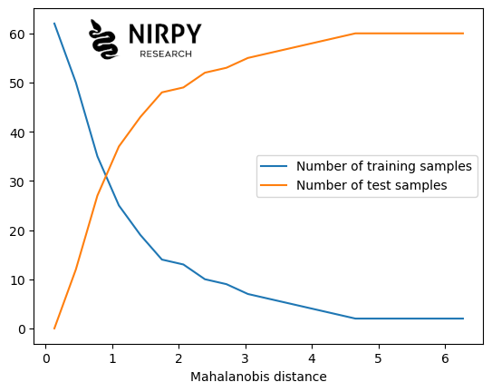
When d is very small, we expect that most samples will be selected, resulting in a large training set. We can then increase d in steps and as we do so, the number of selected samples will decrease. We can choose to stop once the number of selected samples will change little between consecutive iterations, or if it drops below a specified value (for instance 75% of the total dataset).
A Python implementation of the Puchwein algorithm
As for the case of the SPXY algorithm, the efficient calculation of pairwise distances is done using the combination of two functions available from SciPy: pdist and squareform. Let’s start with importing the required libraries and loading a dataset
|
1 2 3 4 5 6 7 8 9 10 11 |
import numpy as np from sklearn.decomposition import PCA import pandas as pd from scipy.spatial.distance import pdist, squareform import matplotlib.pyplot as plt url = 'https://raw.githubusercontent.com/nevernervous78/nirpyresearch/master/data/Incombustible_Material_NIR.csv' data = pd.read_csv(url) X = data.values[:,2:] y = data["TIC Value"].values |
The essence of the Puchwein algorithm is to carry out a PCA decomposition, and then calculate pairwise Mahalanobis distance on the resulting PCA scores.
In this example, I set the number of principal components to 5, but the value can be chosen according to your dataset (you can check the variance explained, for instance).
|
1 2 3 4 5 6 7 8 9 10 11 12 13 14 |
n_components = 5 pca = PCA(n_components=n_components) scores = pca.fit_transform(X) # Pairwise Mahalanobis distances in score space dist_matrix = squareform(pdist(scores, metric='mahalanobis')) fig, ax = plt.subplots() ax.set_aspect('equal') img = ax.imshow(dist_matrix) ax.set_xlabel("Sample number") ax.set_ylabel("Sample number") ax.set_title("Pairwise Mahalanobis distance") fig.colorbar(img) |
To give you a feeling, here’s how the distance matrix looks like, if we colour-code its values.
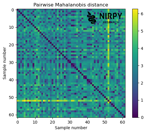
The elements on the diagonal are all zeros, which is the distance of each sample from itself. The matrix is triangular, as you would expect since the distance of sample A from sample B is the same as the distance of sample B from sample A, etc.
Here’s the main function implementing the Puchwein algorithm. Let’s write it down and then discuss the important bits.
|
1 2 3 4 5 6 7 8 9 10 11 12 13 14 15 16 17 18 19 20 21 22 23 24 25 26 27 |
def select_training_puchwein(distance_matrix, distance): # Distance from centroid ≈ average distance to all other points centroid_dist = np.mean(distance_matrix, axis=1) # Start with the farthest sample from the centroid sampling_order = np.argsort(-centroid_dist) # Calculate min and max values of the distance matrix min_distance, max_distance = distance_matrix[distance_matrix != 0].min(), \ distance_matrix[distance_matrix != 0].max() # Initialise list of training indices train_indices = [] # Array to track the distance of each samples from the already selected. # Initially set to the max distance. min_dist_to_selected = np.full(distance_matrix.shape[0], max_distance) for idx in sampling_order: # Loop to select samples that are >= distance if min_dist_to_selected[idx] >= distance: train_indices.append(idx) # Update running minimum distances d = distance_matrix[idx] min_dist_to_selected = np.minimum(min_dist_to_selected, d) # The difference between the array of all indices and the training indices is the array of the test indices test_indices = np.setdiff1d(np.arange(distance_matrix.shape[0]), train_indices) return (train_indices, test_indices) |
The function takes the distance matrix and the user-specified threshold distance ( distance) as inputs. The first two lines select the sampling order (in which order we go through the samples in the dataset), by sorting the samples according to decreasing distance from the centroid. This is important because we want the training set to cover the maximum data span, hence we want to start from the largest distance.
Next, we need to check if each sample is far enough (i.e. at a distance that is at least d ) from already selected samples. This is done by keeping track of the minimum distance that each sample has from selected ones, in the 1D array min_dist_to_selected . This array is initialised with all its values equal to the maximum distance. When an element is selected (i.e. it is added to the pool of selected samples), the min_dist_to_selected array is updated by selecting the element-wise minimum with that sample’s row in the distance matrix.
At the end of the loop, the array of test indices is calculated by taking the difference between the entire list of indices and the ones selected for training, with the setdiff1d function of Numpy.
In the implementation above, the select_training_puchwein function loops once through all the samples and select those that are at a distance at least d from one another. By fixing d we don’t know a priori how many samples will be selected in the training set. For instance, running this code:
|
1 2 |
training_indices, test_indices = select_training_puchwein(dist_matrix, 2) print(len(training_indices), len(test_indices)) |
Returns the values 13 and 49, i.e. 13 samples are selected to be part of the training set.
Selecting the number of samples
To get an idea of the number of samples selected in each set, as a function of the distance threshold, do the calculation in a loop
|
1 2 3 4 5 6 7 8 9 10 11 12 13 14 15 16 |
min_distance, max_distance = dist_matrix[dist_matrix != 0].min(), \ dist_matrix[dist_matrix != 0].max() n_steps = 20 n_train, n_test = np.zeros(n_steps),np.zeros(n_steps) dist_steps = np.linspace(min_distance, max_distance,n_steps) for i, distance in enumerate(dist_steps): training_indices, test_indices = select_training_puchwein(dist_matrix, distance) n_train[i] = len(training_indices) n_test[i] = len(test_indices) plt.plot(dist_steps, n_train, label = "Number of training samples") plt.plot(dist_steps, n_test, label = "Number of test samples") plt.xlabel("Mahalanobis distance") plt.legend() plt.show() |
Distribution of training samples in score space
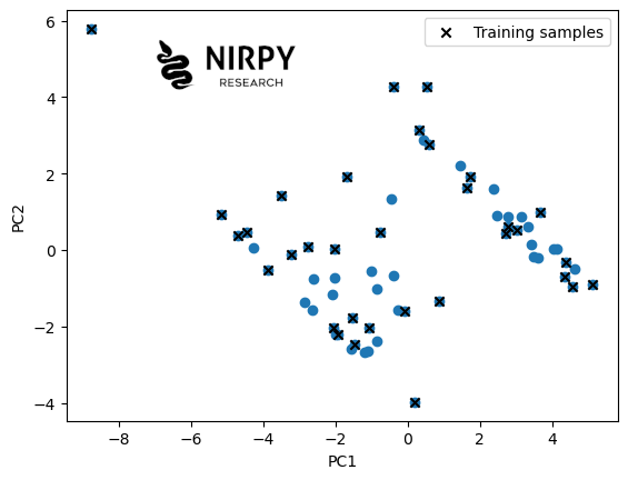
Here’s an example on how to check which samples are selected in the training set, for a given value of the distance threshold. The example shows the samples in the score plot of the first two principal components.
|
1 2 3 4 5 6 7 |
training_indices, test_indices = select_training_puchwein(dist_matrix, 0.9) plt.scatter(scores[:,0], scores[:,1]) plt.scatter(scores[training_indices,0], scores[training_indices,1], marker='x', color='k', label = 'Training samples') plt.legend() plt.xlabel('PC1') plt.ylabel('PC2') plt.show() |
An interesting application of the Puchwein algorithm
Imagine we want to build a calibration model using near-infrared spectra. To do so, we need to measure a reference property of the samples already measured by NIR. The thing is that acquiring NIR spectra is usually much quicker and inexpensive that measuring reference properties.
Therefore, we could decide to screen a lot of samples using NIR, then use the Puchwein algorithm to decide which samples are going to be measured for the reference values. Under the assumption that the distance between the spectra (in the sense of the Puchwein algorithm) is proportional to the difference between the reference values, this will enable us to select the subset of samples that will give us the best coverage of the reference values.
To show a practical example, let’s use NIR data taken from the paper In Situ Measurement of Some Soil Properties in Paddy Soil Using Visible and Near Infrared Spectroscopy by Ji Wenjun et al. The data is available here.
|
1 2 3 4 5 |
# Load data and define arrays data = pd.read_excel("/home/rubens/MEGA/Nirpy/data/File_S1.xlsx") X = data.values[1:,8:].astype('float32') wl = np.linspace(350, 2500, X.shape[1]) y = data["TOC"].values[1:].astype("float32") |
These are 184 NIR spectra of soil samples and associated value of Total Organic Carbon (TOC). Let’s pretend we didn’t know the reference value of the TOC, and we only could measure it for a subset of samples. Which ones do we pick? Let’s run the Puchwein algorithm and find out.
|
1 2 3 4 5 6 7 8 9 10 11 12 13 14 |
n_components = 3 pca = PCA(n_components=n_components) scores = pca.fit_transform(X) dist_matrix = squareform(pdist(scores, metric='mahalanobis')) min_distance, max_distance = dist_matrix[dist_matrix != 0].min(), \ dist_matrix[dist_matrix != 0].max() training_indices, test_indices = select_training_puchwein(dist_matrix, 1) plt.scatter(scores[:,0], scores[:,1]) plt.scatter(scores[training_indices,0], scores[training_indices,1], marker='x', color='k', label = 'Training samples') plt.legend() plt.xlabel('PC1') plt.ylabel('PC2') plt.show() |
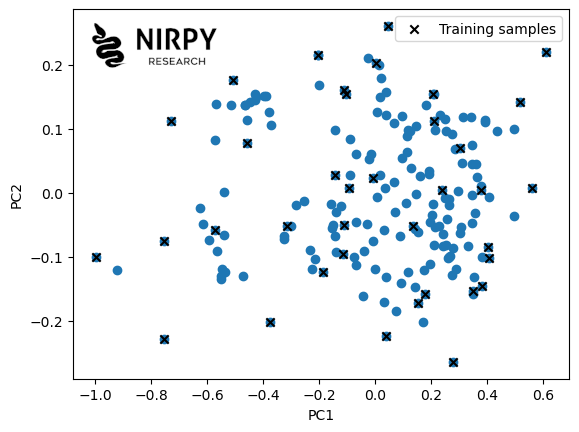
Setting the threshold distance to 1, the algorithm selects 37 samples (out of 184), and this is their distribution in the score space.
Importantly, here’s the distribution of the reference values of this subset, compared to the reference values of the entire set
|
1 2 3 4 5 6 7 8 9 10 |
# Fix the bin size to compare the two histograms binwidth = 1 bins=np.arange(min(y), max(y) + binwidth, binwidth) plt.hist(y, bins=bins) plt.hist(y[training_indices], bins=bins, label = 'Selected samples') plt.xlabel("Reference TOC") plt.ylabel("Number of samples") plt.legend() plt.show() |
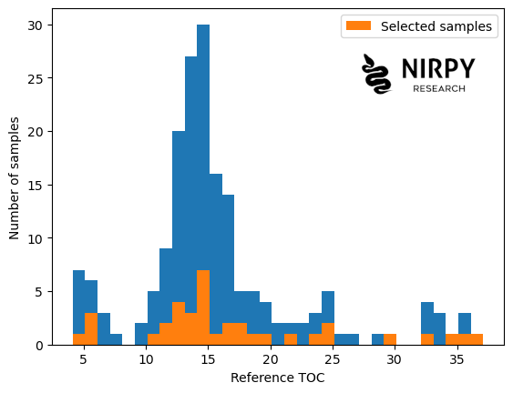 The selected samples cover the full range of TOC values, despite most of the samples in the original set are clustered around TOC values between 10 and 20. In this example, the Puchwein algorithm helps us designing our experiment in the optimal way, given the constraints on measuring values.
Thanks for reading and until next time!
Daniel
References
[1] G. Puchwein (1988). Selection of calibration samples for near-infrared spectrometry by factor analysis of spectra. Analytical Chemistry, 60, 569–573.
[2] See also the R implementation of the Puchwein algorithm. R: Puchwein algorithm for calibration sampling.
**
The feature image is a posterized rendering of an original photo by the author.