
The Concordance Correlation Coefficient (CCC) was introduced by Lawrence Lin in 1989. It was developed as a further metric (in addition to the usual Pearson correlation coefficient) to quantify the similarity between two sets of data, for instance a gold standard and a second reading.
The CCC can be informative for the quantification of regression results in spectroscopy. In this post we are going to define it and compare it with other well known correlation measures: the Pearson correlation coefficient and the coefficient of determination R^{2}.
Concordance Correlation Coefficient: definition
The CCC between two variables is defined by
\rho_{c}= \dfrac{2 \sigma_{12}}{(\mu_{1} - \mu_{2})^{2} + \sigma_{1}^{2} + \sigma_{2}^{2}}.We are assuming that we have two variables obeying Gaussian statistics, with mean \mu_{1} and \mu_{2}, and standard deviations \sigma_{1} and \sigma_{2} respectively. The term \sigma_{12} is their covariance.
The CCC can be re-defined in terms of the (Pearson) correlation coefficient:
\rho= \dfrac{\sigma_{12}}{\sigma_{1} \sigma_{2}}as
\rho_{c} = \rho C.Where C is a bias factor that can be calculated with a bit of algebra from the previous two equations (more details in the first appendix at the end of this post).
The CCC can overcome some of the limitations of the correlation coefficient and provide an alternative metric to the coefficient of determination when, for instance, assessing the quality of a regression model developed with spectral data.
To understand this point, let’s write some simple Python code and evaluate the various coefficients on randomly generated data.
Comparison between CCC and other coefficients
The plan is to calculate CCC, Pearson’s correlation coefficient and the coefficient of determination on synthetic data. We can then the data in a repeatable way so as to understand the influence that the change has on the different coefficients.
Let’s begin with the imports
|
1 2 3 4 5 |
import numpy as np from numpy.random import default_rng import matplotlib.pyplot as plt from sklearn.metrics import r2_score |
Let’s now define the Concordance Correlation Coefficient in a function
|
1 2 3 4 5 |
def ccc(x,y): ''' Concordance Correlation Coefficient''' sxy = np.sum((x - x.mean())*(y - y.mean()))/x.shape[0] rhoc = 2*sxy / (np.var(x) + np.var(y) + (x.mean() - y.mean())**2) return rhoc |
For the sake of this exercise, let’s also define a function calculating the Pearson’s correlation coefficient. There is a ready-made function in Scipy here, if you can’t be bothered, but writing some clear definitions here helps highlighting similarities and differences between the two coefficients.
|
1 2 3 4 5 |
def r(x,y): ''' Pearson Correlation Coefficient''' sxy = np.sum((x - x.mean())*(y - y.mean()))/x.shape[0] rho = sxy / (np.std(x)*np.std(y)) return rho |
Now we can generate synthetic data. We generate an independent variable X of data extracted from a uniform distribution between 0 and 1. The dependent variable Y will be instead extracted from a normal distribution, dependent on the values of X, of which we control two parameters. Here’s the code
|
1 2 3 4 5 6 7 8 9 10 |
rng = default_rng() X = np.random.random_sample(1000) Y = np.zeros_like(X) sigma = 0.01 tilt = 0 for i in range(X.shape[0]): Y[i] = tilt*(X[i]-0.5) + rng.normal(X[i],sigma) print("CCC: %5.5f, rho: %5.5f, R2: %5.5f"%(ccc(X,Y), r(X,Y), r2_score(X, Y))) |
As you can gather, each of the Y values is extracted by a normal distribution whose mean is the corresponding X value. The free parameters are the standard deviation of the Gaussian and a parameter I called “tilt”. A tilt different from zero will introduce a bias in the distribution of Y, which will deviate from the nominal 45 degree line when plotted against X.
Let’s see a few examples (the code for the plot is copied at the end of this post). In this first batch of examples we are only going to vary the standard deviation, keeping the tilt=0.
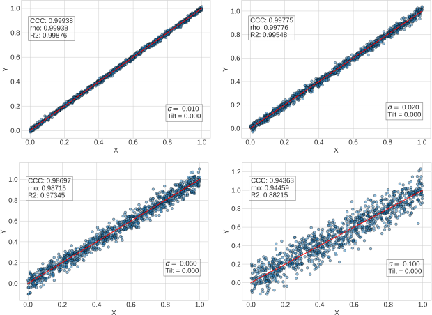
The values of the parameters are copied at the bottom right of each plot. The calculated value of the coefficients at the top left. Let’s look at what’s happening here. As we increase \sigma , the Y data gets more and more spread over. They do however (on average) follow the 45 degree line when plotted against X. Of the three coefficients, R^{2} is the one that decreases the most.
The coefficient of determination measures the amount of variance in Y that is explained by X. When we increase the \sigma we are introducing a source of variability that is external to X, and this has a more deleterious effect on R^{2} that on the other correlation coefficients. Both Pearson’s and CCC go hand in hand in the four examples above. Both measure the fact that there is a linear correlation between the data which gets only mildly worse with increasing \sigma .
The situation changes when we vary the tilt. Take a look.

By increasing the tilt we introduce a bias, so that the Y values do not sit on the 45 degree line any longer. The coefficient of determination, not surprisingly, plunges since less and less of the variance of Y is eventually “explained” by X.
Interestingly the Pearson’s correlation coefficient instead doesn’t budge. In fact it marginally grows as the relative standard deviation of the data is decreasing since we are increasing the range of the Y values. There is an obvious correlation between the X and Y variables, and the Pearson’s correlation coefficient highlights that.
The behaviour of the CCC is somewhere in between these two extremes. As the tilt increases the CCC obviously decreases, but not as markedly as R^{2}. Even in the worst case scenario (bottom right graph of the previous figure) the CCC is still sitting at around 0.8.
The reason is that, just like for the Pearson’s correlation coefficient, the CCC keeps track of the strong linear relation between X and Y. It does however also keep track of the fact that such a linear relation doesn’t line up with the 45 degree line. In other words, X and Y are linearly correlated by the 45 degree line is a “bad fit” for that relation.
The situation exemplified here is not uncommon when trying to produce regression models from spectroscopy data. This is obviously a toy model, but you may recognise the situation in which, after the regression is fitted, the prediction data shows a correlation that doesn’t sit exactly on the 1:1 line. In this case, keeping track of the Concordance Correlation Coefficient, may be a useful indicator way to optimise the model.
That’s us for today. Thanks for reading and until next time.
Appendix: the bias factor C
The Concordance Correlation Coefficient is defined as
\rho_{c}= \dfrac{2 \sigma_{12}}{(\mu_{1} - \mu_{2})^{2} + \sigma_{1}^{2} + \sigma_{2}^{2}},while the correlation coefficient is
\rho= \dfrac{\sigma_{12}}{\sigma_{1} \sigma_{2}}.By comparing the two equations, you can work out that by defining the factor
C= \dfrac{2 \sigma_{1} \sigma_{2}}{(\mu_{1} - \mu_{2})^{2} + \sigma_{1}^{2} + \sigma_{2}^{2}},we obtain: \rho_{c} = \rho C.
Now, C is always positive and less than 1. Its maximum value is reached when the two variables have identical mean and standard deviation. For instance, if we extract two sets of random numbers from the same Gaussian distribution, and we build a scatter plot of one set against the other, we’ll obtain a plot that is very similar to the top-left plot in the first figure above. That is, the values will be different, but the line of best fit will be essentially at 45 degrees.
On the contrary, if the means of the two distributions are different, than we have a tilt (as defined above) that is non-zero and the line of best fit will be at angle that is not 45 degrees.
Appendix: Python code to generate the graphs
|
1 2 3 4 5 6 7 8 9 10 11 12 13 14 15 16 17 18 19 20 |
with plt.style.context(('seaborn-whitegrid')): plt.figure(figsize=(8,6)) # Scatter plot of X vs Y plt.scatter(X,Y,edgecolors='k',alpha=0.5) # Plot of the 45 degree line plt.plot([0,1],[0,1],'r') plt.text(0, 0.75*Y.max(), "CCC: %5.5f"%(ccc(X,Y))+"\nrho: %5.5f"%(r(X,Y))+"\nR2: %5.5f"%(r2_score(X, Y)),\ fontsize=16, bbox=dict(facecolor='white', alpha=0.5)) plt.text(0.8, 0.1, "$\sigma=$ %5.3f"%(sigma)+"\nTilt = %5.3f"%(tilt),\ fontsize=16, bbox=dict(facecolor='white', alpha=0.5)) plt.xticks(fontsize=16) plt.yticks(fontsize=16) plt.xlabel('X',fontsize=16) plt.ylabel('Y',fontsize=16) plt.show() |
Featured image credit: Johannes Plenio.


