A short while ago, I received a very interesting question from one of our readers: is there an objective way to optimise the choice of parameters for Savitzky–Golay (SG) smoothing? Other than judging by eye, is there (loosely speaking) a recipe to decide what level of smoothing is just enough? A great question. In our previous post we discussed how to implement a SG smoothing, and briefly discussed how to go about choosing the parameters. It’s time to get into that in more detail.
To understand the rationale behind the choice of parameters, let’s take a step back and refocus on why we want to smooth our data. The purpose of smoothing is to get rid of random noise while (ideally) preserving the true spectral signal. Therefore, the original question about the optimal choice of smoothing parameters can be rephrased as: “How can we tell the signal from the noise?”
To state the obvious, it is hard to come up with a recipe that is going to work in every situation. We can however devise a methodology that can guide us towards an objective decision about the amount of smoothing to apply. In this tutorial I will tell you about the method I follow, and the reason behind it. It is by no means a prescriptive method – there is always an amount of personal judgement involved, but it serves well as a guideline for the process.
My method is based on the analysis of the power spectrum associated with our signal. In what follows we are going to describe what a power spectrum is and how we can use it to understand the amount of smoothing to apply. As in our original post on smoothing, the data is taken from J. Cuadros and collaborators: Abundance and composition of kaolinite on Mars: Information from NIR spectra of rocks from acid-alteration environments, Riotinto, SE Spain. The dataset is freely available for download here.
Understanding the power spectrum
The power spectrum of a signal is the square modulus of its Fourier Transform. We introduced the Fourier spectral smoothing method in a previous post, where we applied specific filters in Fourier space to generate derivatives and smoothed versions of the original spectrum. We haven’t however discussed the concept of power spectrum at all. Now it’s time to do that.
First of all, a few remarks about the terminology. The word ‘spectrum’ in the power spectrum may be confusing here because it happens to be the same word describing the original signal we want to smooth (for instance an NIR spectrum). Fourier Transforms are traditionally applied to time-dependent signals, for instance a time-varying electrical oscillation in a circuit or a sound wave. The ‘spectrum’ of such signals indeed represents the amount of energy for each frequency of the time-dependent signal. The ‘pitch’ of a sound is the frequency associated with it. Therefore the square modulus of the Fourier Transform of such a signal is traditionally called power spectrum.
In our case we are already dealing with a spectrum. Sure enough our spectra (NIR, MIR, Raman, fluorescence, etc) are the consequence of some time-varying oscillation associated with molecules in our samples. For instance various vibrational modes of molecules are associated with specific time-dependent motion patterns of such molecules, leading to specific frequencies being absorbed or emitted. Therefore the square modulus of its Fourier transform is not technically a ‘spectrum’ (should be a time-dependent signal in fact!) but we stick with the conventional terminology and call it power spectrum. The important thing is to understand what we are talking about.
Good, now that we explain our use of the terminology, let’s write the code to calculate the power spectrum. As usual, we put the entire snippet here and we’ll go through it step by step below.
|
1 2 3 4 5 6 7 8 9 10 11 12 13 14 15 16 17 18 19 20 21 22 23 24 25 26 |
import numpy as np import pandas as pd import matplotlib.pyplot as plt from scipy.signal import savgol_filter, general_gaussian data = pd.read_excel('NIR data Earth analogs.xlsx') X = data['C1'].values wl = data['nm'].values # Calculate the power spectrum ps = np.abs(np.fft.fftshift(np.fft.fft(X)))**2 # Define pixel in original signal and Fourier Transform pix = np.arange(X.shape[0]) fpix = np.arange(ps.shape[0]) - ps.shape[0]//2 with plt.style.context(('ggplot')): fig, axes = plt.subplots(nrows=1, ncols=2, figsize=(12, 6)) axes[0].plot(pix, X) axes[0].set_xlabel('pixel') axes[0].set_ylabel('NIR spectrum') axes[1].semilogy(fpix, ps, 'b') axes[1].set_xlabel('pixel (Fourier space)') axes[1].set_ylabel('Power Spectrum') |
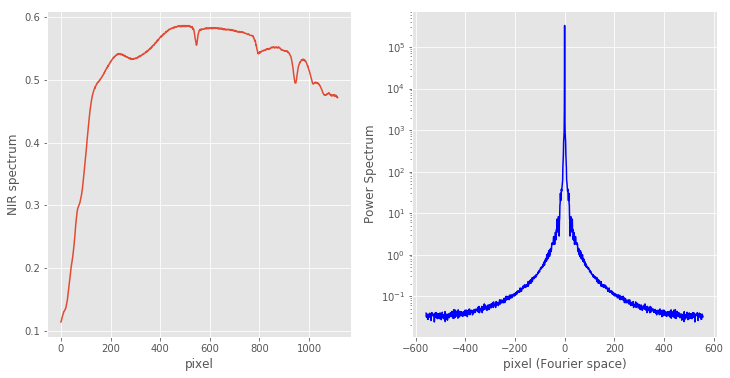
To keep things simple, we avoided using the wavelength information on the x-axis of the first plot. We just plotted the spectrum against the pixel number. The power spectrum, as discussed, is simply the square of the absolute value of the Fourier Transform of the signal.
A short digression here is in order. Generally, the Fourier Transform of any signal is a complex-valued function. That means that it has a real and an imaginary part. That is why, in order to plot it on a real axis (the pixel value) we have to take the absolute value of it. Now, it turns out – for reasons we are not going to discuss here – that the Fourier transform of a (real-valued) signal of size N (N pixels) has only N/2 independent values. You can see in the second plot that the power spectrum is symmetric with respect to the central point.
That is the reason we have used two tricks: 1) we shifted the array by half its length with the np.fft.fftshift function. 2) We have specifically defined fpix, as the pixel in Fourier space.
In this way the power spectrum values close to the central point (fpix close to zero) correspond to the ‘low frequencies’ of our signal, i.e. the amount of signal associated with slowly varying parts of the spectrum. Conversely, the ‘high frequency’ part of the power spectrum is associated with the fast moving regions of the original signal. Note that we have plotted the power spectrum as a lin-log plot, to be able to visualise the large range of variation of the power spectrum.
Choosing the optimal smoothing parameters
This is the absolute key point of this tutorial. Our aim is to tell the signal from the noise. The noise (if it’s truly random) will change randomly from pixel to pixel, thereby giving rise to high frequency components in the power spectrum. The signal intensity on the other hand, is mostly concentrated in the lower frequency range, even though it may still feature sharp peaks, such as in MIR or Raman.
Following this idea, I typically choose a featureless region of the original spectrum and calculate its power spectrum only in that region. For our data, I’m going to pick the region between pixel 600 and 750.
|
1 2 3 4 5 6 7 8 9 10 11 12 13 14 15 16 |
# Calculate the power spectrum ps = np.abs(np.fft.fftshift(np.fft.fft(X[600:750])))**2 # Define pixel in original signal and Fourier Transform pix = np.arange(X[600:750].shape[0]) fpix = np.arange(ps.shape[0]) - ps.shape[0]//2 with plt.style.context(('ggplot')): fig, axes = plt.subplots(nrows=1, ncols=2, figsize=(12, 6)) axes[0].plot(pix, X[600:750]) axes[0].set_xlabel('pixel') axes[0].set_ylabel('NIR spectrum') axes[1].semilogy(fpix, ps, 'b') axes[1].set_xlabel('pixel (Fourier space)') axes[1].set_ylabel('Power Spectrum') |
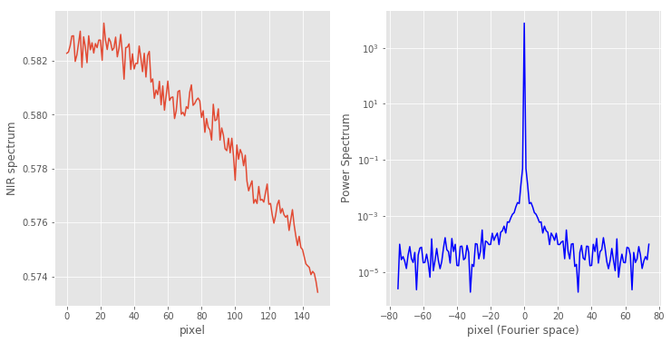
In this region the original spectrum changes little (about 1% in fact), therefore its power spectrum is clumped in a small region of about 20 pixels in the low frequency range. The rest is pretty much random noise.
This is the ideal power spectrum to test the smoothing parameters of our SG filter, or to set the window size of our Fourier filter. The recipe for a SG filter is as follows.
- Calculate 2-3 different smoothed spectra, with different parameters of the SG function.
- Calculate the power spectrum of a relatively featureless region of the spectrum, in both the original and the smoothed versions.
- Compare the power spectra in a lin-log plot.
Here’s the code
|
1 2 3 4 5 6 7 8 9 10 11 12 13 14 15 16 17 18 19 20 21 22 23 24 25 |
# Set some reasonable parameters to start with w = 5 p = 2 # Calculate three different smoothed spectra X_smooth_1 = savgol_filter(X, w, polyorder = p, deriv=0) X_smooth_2 = savgol_filter(X, 2*w+1, polyorder = p, deriv=0) X_smooth_3 = savgol_filter(X, 4*w+1, polyorder = 3*p, deriv=0) # Calculate the power spectra in a featureless region ps = np.abs(np.fft.fftshift(np.fft.fft(X[600:750])))**2 ps_1 = np.abs(np.fft.fftshift(np.fft.fft(X_smooth_1[600:750])))**2 ps_2 = np.abs(np.fft.fftshift(np.fft.fft(X_smooth_2[600:750])))**2 ps_3 = np.abs(np.fft.fftshift(np.fft.fft(X_smooth_3[600:750])))**2 # Define pixel in Fourier space fpix = np.arange(ps.shape[0]) - ps.shape[0]//2 plt.figure(figsize=(10,8)) with plt.style.context(('ggplot')): plt.semilogy(fpix, ps, 'b', label = 'No smoothing') plt.semilogy(fpix, ps_1, 'r', label = 'Smoothing: w/p = 2.5') plt.semilogy(fpix, ps_2, 'g', label = 'Smoothing: w/p = 5.5') plt.semilogy(fpix, ps_3, 'm', label = 'Smoothing: w/p = 3.5') plt.legend() plt.xlabel('pixel') |

Discussion
As mentioned, the power spectrum is significant within a region of about 20 pixels from the centre. At that level it has already dropped by about 8 orders of magnitude from its maximum point. After that level the power spectrum is nearly constant, which gives us an indication about the power spectrum of random noise.
Therefore, we would like that the power spectrum of the smoothed signal is overlapping with the original one within the 20 pixel region, but not much more. After the 20th pixel we would like to see the power spectrum being significantly smoothed by the application of the SG filter. (Incidentally, if we were working with a Fourier smoothing, we’d set the width of our window to about 20 pixels).
The red curve in the plot above, the red curve (w/p = 2.5) is clearly not smoothing enough, as it is still oscillating quite strongly after 20 pixels. To discriminate between green and magenta, we need to zoom in towards that central region. This is done simply by adding the command plt.xlim((0,30)) right before the xlabel command. Here’s the result

The difference is really tiny, but you can notice that the green curve tends to differ slightly from the original before the 20 pixel mark. The magenta curve on the other hand does what we’d like to see, i.e. it tracks closely the original signal within the 20 pixels and smooths it afterwards.
An here’s the result of the action of the three filters on the original data
|
1 2 3 4 5 6 7 8 9 10 |
plt.figure(figsize=(9,6)) interval = np.arange(530,570) with plt.style.context(('ggplot')): plt.plot(wl[interval], X_smooth_1[interval], 'r', label = 'Smoothing: w/p = 2.5') plt.plot(wl[interval], X_smooth_2[interval], 'g', label = 'Smoothing: w/p = 5.5') plt.plot(wl[interval], X_smooth_3[interval], 'm', label = 'Smoothing: w/p = 3.5') plt.xlabel("Wavelength (nm)") plt.ylabel("Second Derivative Reflectance") plt.legend() plt.show() |

Conclusion
In this tutorial I’ve discussed the method I often use to estimate the optimal parameters of a Savitzky–Golay smoothing filter. The trick is to look at a portion of the spectrum which is, as much as possible, devoid of important features. That would enable a reasonable estimate of the noise level in the spectrum by means of the ‘power spectrum’, which is the squared magnitude of the Fourier transform of the original spectrum. Subtle changes in the S-G parameters can be visualised in the power spectrum, as a way to more objectively set the optimal smoothing for your spectra.
If you found this post useful, go ahead and share it with friends and colleagues, and I’ll promise you my eternal gratitude!
Until next time.